Section
0A. Scope And Document Basis
This page documents the technical logic of the CPT interpreter from raw CPT file import through Stage 6 engineering use. It is written as a theory-and-implementation note: formulas, classifications, parameter routes, engineering assumptions, and the principal references behind the current application.
0A.1 Coverage
The documentation covers the current implemented workflow: CPT file parsing for GEF, Excel, and CSV sources, per-point CPT classification, layer detection, layer parameter assignment, stiffness derivation, experimental m-fitting, and the Stage 6 engineering applications.
Where the application contains an engineering simplification, the simplification is stated explicitly. The purpose is not to replace engineering judgement, but to make the implemented mathematics auditable and readable.
- Classification and boundary logic are documented separately from parameter assignment.
- Stage 6 uses the interpreted CPT state produced by the earlier stages rather than reclassifying the profile independently.
- The notation below follows geotechnical convention with compression positive and depth measured downward.
0A.2 Layer quantities carried into engineering use
Per interpreted layer, the application carries the quantities needed by the engineering modules: top and bottom depth, γ and γsat, φ′, c′, cu, Eoed,ref, Eoed,i, E50,ref, Eur,ref, m, K0,nc, νur, kh, and kv.
Geometry, load combination, hydraulic scenario, and optional Stage 5 tuning are then applied on top of those layer values.
Primary references: EN 1997-1:2004+A1:2013; NBN EN 1997-1 ANB:2022.
Section
1. Stage 1 — CPT File Loading
The first stage reconstructs a usable CPT dataset from the uploaded source file. Rich GEF files and Excel workbooks with Header/Data sheets are preferred because they carry metadata, water level, surface level, and coordinates. Minimal CSV files are also accepted when only the measurement trace is available.
1.1 Supported file structures and column mapping
GEF files declare their physical quantities through #COLUMNINFO lines. The application reads the quantity identifier and maps it to the relevant column index; column order is therefore never assumed.
Excel workbooks are read from a Data sheet and, when present, a Header sheet. The Data sheet may contain depth, qc, fs, and Rf; the Header sheet can provide project, test, location, date, water level, surface level, coordinates, and the net area ratio.
CSV files are the reduced-input route. They must contain headers named depth and qc. Optional headers are fs and rf. Comma, semicolon, and tab delimiters are detected automatically.
A recommended minimal CSV header is depth [m], qc [MPa], fs [MPa]. If decimal commas are used in the values, a semicolon-delimited CSV is recommended.
- GEF quantity 1: penetration length.
- GEF quantity 2: qc.
- GEF quantity 3: fs.
- GEF quantity 4: Rf.
- GEF quantity 6: u2.
- GEF quantity 11: corrected depth, used before quantity 1 when both are present.
- Excel/CSV column headers may include units, for example
qc [MPa],fs kPa, orFriction ratio (Rf) in %.
1.2 Unit conversion and row filtering
The parser converts qc and fs to MPa based on the declared GEF unit string or the Excel/CSV column header. Headers containing MPa are used directly; kPa is divided by 1000; Pa is divided by 1 000 000.
If the unit declaration is absent or ambiguous, a heuristic fallback is used so the file remains workable: qc values above 100 are treated as kPa, otherwise MPa; fs values above 1000 are treated as Pa, values above 10 as kPa, otherwise MPa. Explicit unit labels are therefore strongly recommended.
Rows are removed when they clearly do not represent meaningful CPT measurements, namely negative depths, values before cone engagement, or all-zero terminal rows.
- qc
- cone resistance [MPa]
- fs
- sleeve friction [MPa]
- Rf
- friction ratio [%]
- u2
- pore pressure behind the cone [MPa]
- Depth is expected in metres below surface.
- Rf is optional; when absent or invalid, the app computes it from fs and qc.
- Rows with z < 0 are discarded.
- Rows with qc < 0.02 MPa are treated as cone-not-engaged and discarded.
- All-zero rows appended by logging software are discarded.
1.3 Water table, elevation, and header metadata
The phreatic level is first taken from the GEF measurement variables or the Excel Header field Waterniveau when available; otherwise a default depth below surface is assigned. CSV files do not carry this metadata, so the engineer should review or override the default after import.
Surface elevation is read from the GEF ZID header, the Excel Header field Grondniveau, or entered manually. When present, all depth values can be expressed relative to TAW as well as depth below surface.
- zTAW
- elevation relative to TAW [m]
- zsurface
- surface elevation [m TAW]
- z
- depth below surface [m]
Section
2. Stage 2 — Classification
Classification is applied per CPT reading rather than per final layer. The result is a behavioural or code-based soil type sequence that later controls where layer boundaries fall.
2.1 Robertson (1990) — normalized SBT / Ic
The Robertson route uses a normalized qt–Fr framework. Because final layer unit weights are not yet available at Stage 2, the app uses a preliminary stress estimate with fixed unsaturated and saturated unit weights.
If pore pressure u2 and net area ratio a are available, the cone resistance is corrected to qt; otherwise the measured qc is used directly.
- a
- net area ratio [-]
- qt
- corrected cone resistance [MPa]
- fs,eff
- effective sleeve friction used in normalization [MPa]
- Qt
- normalized cone-resistance parameter [-]
- Fr
- normalized friction ratio [%]
- Ic
- soil behaviour type index [-]
- The current app groups the normalized result into Gravel, Sand, Silty sand, Sandy clay, Clay, and Peat / organic.
- Sensitive fine-grained soil is not inferred separately from Ic alone.
2.2 Robertson (2016) — iterative normalized SBT / Qtn
The Robertson 2016 route keeps the same broad SBT / Ic family mapping as the earlier normalized Robertson workflow, but replaces the fixed-stress-exponent cone normalization with the iterative Qtn formulation. The stress exponent n varies with the inferred soil behaviour and is solved iteratively.
This route may be preferred when the input is a CPTu, but the implementation does not require measured u2. If u2 is absent, the app uses qt = qc in the same way as the Robertson 1990 fallback.
- Qtn
- stress-normalized cone-resistance parameter with variable exponent [-]
- n
- stress exponent solved iteratively from soil behaviour [-]
- pa
- atmospheric reference pressure = 100 kPa
- The implementation reuses the existing broad app families: Gravel, Sand, Silty sand, Sandy clay, Clay, and Peat / organic.
- The displayed method metric is Qtn; the Ic boundaries remain the same as the Robertson 1990 route.
2.3 CUR 3 layers — broad qc–Rf zoning
The CUR 3 layers route is implemented as a direct qc–Rf zoning rule based on the published broad chart with four material fields: Sand, Silt, Clay, and Peat. It is a boundary-generation method, not a detailed parameter catalogue.
The implementation follows the chart as nested zones checked from the most specific region to the broadest envelope: sand first, then silt, then clay, with peat as the remaining outside region.
To keep the downstream parameter workflow stable, the chart field “Silt” is carried internally as the app’s intermediate family and tagged with the subtype marker CUR3 silt. The chart logic itself remains four-zoned.
- qc
- measured cone resistance [MPa]
- Rf
- measured friction ratio [%]
Show published CUR 3 chart
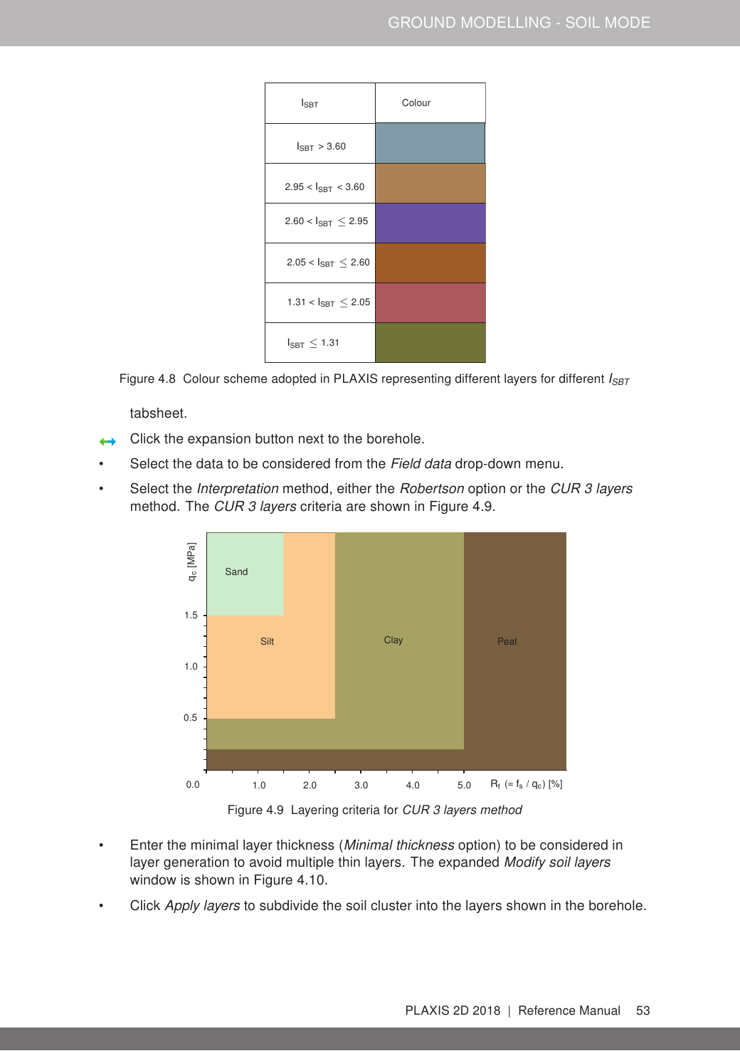
- This route is direct and non-normalized: no stress correction is applied to qc before classification.
- The current app uses this route for broad layer boundary logic; detailed geotechnical parameter assignment is still handled later by the Stage 3 parameter method.
- Internal mapping note: the chart field “Silt” is stored as the app’s intermediate type family so that later parameter and compatibility tables remain usable.
2.4 NEN 6740 — stress-dependent material classification
NEN 6740 uses a stress-corrected cone resistance together with friction ratio. The source method is graphical: a semilog chart with fourteen material areas rather than a closed algebraic decision tree.
The app therefore separates the method into two parts. First it evaluates the published stress correction documented in the Deltares D-SHEET Piling manual. Then it applies a transparent representative-area rule that selects the nearest material area from a digitized fourteen-material set.
- qc,NEN
- stress-corrected cone resistance used by the NEN chart [MPa]
- σ′v0
- initial effective vertical stress at the CPT reading [kPa]
- s
- implemented chart-coordinate projection used for the representative-area search [-]
- sj
- projected coordinate of representative material area j [-]
Show published NEN 6740 chart
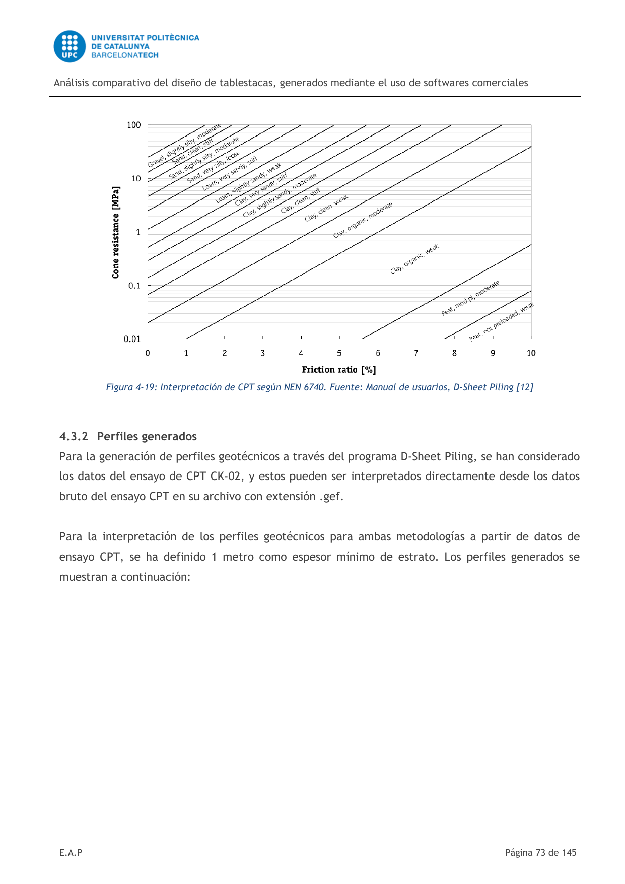
- The stress-correction equation with exponent 0.67 is part of the documented Deltares implementation of the published NEN route; the one-dimensional score projection is the app’s deterministic way of reproducing the graphical chart.
- The score coefficient magnitude 0.34 is not a normative NEN coefficient. It is the regression-fit semilog projection magnitude through the fourteen stored representative centres used by the app.
- The representative materials are: gravel, slightly silty, moderate; sand, clean, stiff; sand, slightly silty, moderate; sand, very silty, loose; loam, very sandy, stiff; loam, slightly sandy, weak; clay, very sandy, stiff; clay, slightly sandy, moderate; clay, clean, stiff; clay, clean, weak; clay, organic, moderate; clay, organic, weak; peat, moderately preloaded, moderate; peat, not preloaded, weak.
- The weakest transition remains the area-5/area-6 pair (loam, slightly sandy, weak versus clay, very sandy, stiff). Near ties are resolved by the fixed chart order of the stored representative set.
- A repo verification script re-projects all fourteen centres at several effective stresses to ensure the stored centres and the implemented score formula stay in sync.
- The selected NEN material is then mapped into the app’s internal type families so that later layer grouping and parameter workflows remain consistent.
2.5 NEN Tabel 3 — direct subtype classification
The Table 3 route uses raw qc and Rf and returns a detailed subtype together with the characteristic parameter row used later in the workflow. The direct source documented here is the implemented NEN Tabel 3 catalogue itself, not a separate Eurocode classification chart.
Because the table contains overlapping qc–Rf envelopes, the app evaluates the rows deterministically in table order rather than assuming the source is mutually exclusive. The implemented family order is grind, zand, leem, klei, then veen. Within each family, subrows are checked top-to-bottom, with qc lower bounds inclusive and upper bounds exclusive. For Rf, the open bands Rf < 1 and Rf > 6 remain strict, while the bounded intervals are treated as closed.
For this method, the raw boundary logic follows the detailed subtype result rather than only the broad family. This means subtype changes such as density or consistency transitions inside one family can create provisional layer boundaries before smart merge and minimum-thickness correction simplify them.
- qc
- measured cone resistance [MPa]
- Rf
- measured friction ratio [%]
- γ
- unit weight above the phreatic level [kN/m³]
- γsat
- unit weight below the phreatic level [kN/m³]
- φ′
- effective friction angle [°]
- c′
- effective cohesion [kPa]
- cu
- undrained shear strength [kPa]
Implemented NEN Tabel 3 rows used by the direct subtype classifier. The table below is rendered from the active subtype catalogue rather than shown as a synthetic chart.
| Family | Subtype | qc range [MPa] | Rf range [%] | γ [kN/m³] | γsat [kN/m³] | φ′ [°] | c′ [kPa] | cu [kPa] |
|---|---|---|---|---|---|---|---|---|
| Veen | veen, weinig vast | 0.2 ≤ qc < 0.5 | Rf > 6 | 10 | 10 | 15 | 2 | 10 |
| Veen | veen, matig vast | 0.5 ≤ qc < 1.0 | Rf > 6 | 12 | 12 | 15 | 5 | 20 |
| Veen | veen, vast | qc ≥ 1.0 | Rf > 6 | 14 | 14 | 15 | 10 | 40 |
| Klei | klei, weinig vast | 0.4 ≤ qc < 1.0 | 3 ≤ Rf ≤ 6 | 16 | 16 | 20 | 2 | 20 |
| Klei | klei, matig vast | 1.0 ≤ qc < 2.0 | 3 ≤ Rf ≤ 6 | 17 | 17 | 20 | 4 | 50 |
| Klei | klei, vrij vast | 2.0 ≤ qc < 4.0 | 3 ≤ Rf ≤ 6 | 18 | 18 | 20 | 8 | 100 |
| Klei | klei, vast | qc ≥ 4.0 | 3 ≤ Rf ≤ 6 | 19 | 19 | 20 | 15 | 200 |
| Klei zandhoudend | klei (zh), weinig vast | 0.4 ≤ qc < 1.0 | 2 ≤ Rf ≤ 5 | 16 | 16 | 22 | 2 | 20 |
| Klei zandhoudend | klei (zh), matig vast | 1.0 ≤ qc < 2.0 | 2 ≤ Rf ≤ 5 | 17 | 17 | 22 | 4 | 50 |
| Klei zandhoudend | klei (zh), vrij vast | 2.0 ≤ qc < 4.0 | 2 ≤ Rf ≤ 5 | 18 | 18 | 22 | 8 | 100 |
| Klei zandhoudend | klei (zh), vast | qc ≥ 4.0 | 2 ≤ Rf ≤ 5 | 19 | 19 | 22 | 15 | 200 |
| Leem | leem, weinig vast | 0.4 ≤ qc < 1.0 | 2 ≤ Rf ≤ 4 | 17 | 17 | 22 | 0 | 10 |
| Leem | leem, matig vast | 1.0 ≤ qc < 2.0 | 2 ≤ Rf ≤ 4 | 18 | 18 | 22 | 2 | 25 |
| Leem | leem, vrij vast | 2.0 ≤ qc < 4.0 | 2 ≤ Rf ≤ 4 | 19 | 19 | 22 | 4 | 50 |
| Leem | leem, vast | qc ≥ 4.0 | 2 ≤ Rf ≤ 4 | 20 | 20 | 22 | 8 | 100 |
| Zandhoudende leem | leem (zh), weinig vast | 0.4 ≤ qc < 1.0 | 1 ≤ Rf ≤ 3 | 17 | 17 | 25 | 0 | 10 |
| Zandhoudende leem | leem (zh), matig vast | 1.0 ≤ qc < 2.0 | 1 ≤ Rf ≤ 3 | 18 | 18 | 25 | 2 | 25 |
| Zandhoudende leem | leem (zh), vrij vast | 2.0 ≤ qc < 4.0 | 1 ≤ Rf ≤ 3 | 19 | 19 | 25 | 4 | 50 |
| Zandhoudende leem | leem (zh), vast | qc ≥ 4.0 | 1 ≤ Rf ≤ 3 | 20 | 20 | 25 | 8 | 100 |
| Zand | zand, los | 2 ≤ qc < 4 | Rf < 1 | 16 | 18 | 27 | 0 | 0 |
| Zand | zand, matig | 4 ≤ qc < 10 | Rf < 1 | 17 | 19 | 30 | 0 | 0 |
| Zand | zand, dicht | 10 ≤ qc < 15 | Rf < 1 | 18 | 20 | 32 | 0 | 0 |
| Zand | zand, zeer dicht | qc ≥ 15 | Rf < 1 | 18 | 20 | 35 | 0 | 0 |
| Leemhoudend zand | zand (lh), los | 2 ≤ qc < 4 | 1 ≤ Rf ≤ 2 | 16 | 18 | 25 | 0 | 0 |
| Leemhoudend zand | zand (lh), matig | 4 ≤ qc < 10 | 1 ≤ Rf ≤ 2 | 17 | 19 | 27 | 0 | 0 |
| Leemhoudend zand | zand (lh), dicht | 10 ≤ qc < 15 | 1 ≤ Rf ≤ 2 | 18 | 20 | 30 | 0 | 0 |
| Leemhoudend zand | zand (lh), z.dicht | qc ≥ 15 | 1 ≤ Rf ≤ 2 | 19 | 20 | 32 | 0 | 0 |
| Grind | grind, matig | 10 ≤ qc < 20 | Rf < 1 | 18 | 20 | 35 | 0 | 0 |
| Grind | grind, dicht | qc ≥ 20 | Rf < 1 | 19 | 21 | 40 | 0 | 0 |
| Grind klei-/leemhoudend | grind (kh), matig | 10 ≤ qc < 20 | 1 ≤ Rf ≤ 2 | 19 | 21 | 32 | 0 | 0 |
| Grind klei-/leemhoudend | grind (kh), dicht | qc ≥ 20 | 1 ≤ Rf ≤ 2 | 20 | 22 | 37 | 0 | 0 |
All qc limits are applied as lower-inclusive and upper-exclusive. For Rf, the open conditions Rf < 1 and Rf > 6 remain strict; the bounded intervals are treated as closed.
- If no table row matches, the app keeps a deterministic fallback so the workflow can continue, but that fallback is not itself part of Table 3.
- The app UI may still show a legacy “EC7” label because the later parameter workflow is Eurocode-aligned. The direct qc–Rf table documented in this section is the implemented NEN Tabel 3 source.
2.6 Classification versus parameter assignment
Stage 2 is boundary logic only. The classification method decides which soil type each CPT reading belongs to and therefore where soil-type changes occur with depth.
Stage 3 parameter assignment is independent of the chosen classification route. A layer identified by Robertson, CUR 3 layers, or NEN 6740 may still be assigned a Eurocode Table 3 subtype and its associated γ, γsat, φ′, c′, and cu values.
Primary references: Robertson (1990); Robertson (2016); Robertson & Wride (1998); PLAXIS 2D 2018 Reference Manual; NEN 6740; Deltares D-SHEET Piling User Manual; SB260.
Section
3. Stage 3 — Layer Detection And Parameter Assignment
Once every CPT reading carries a classification label from the selected Stage 2 method, the app converts that pointwise sequence into engineering layers in four steps: raw segmentation, optional smart boundary reduction, final minimum-thickness enforcement, and recomputation of the final layer properties from the merged geometry.
3.1 Raw segmentation and boundary placement
The first pass creates provisional raw segments directly from the pointwise Stage 2 classification sequence. For Robertson, CUR 3 layers, and NEN 6740, the raw segment key is the broad internal soil family. For NEN Tabel 3, the raw segment key is the pair {type, subtype}, so detailed subtype changes can create provisional layer boundaries before later simplification.
Boundary depths are then constructed from the retained CPT rows. The first raw segment starts at ground level. Other raw segments start at the midpoint between the last CPT row of the previous segment and the first CPT row of the new segment, unless a downward merge has already handed them an inherited top boundary. If that straddling sample pair is unavailable or degenerate, the app falls back to the legacy 20 mm offset from the first row of the new segment. Segment thickness is always evaluated on these active layer boundaries rather than on the bare difference between first and last CPT reading.
- krow
- raw segmentation key used to decide whether two consecutive CPT rows belong to the same provisional segment [-]
- zlast row,prev, zfirst row,curr
- last retained CPT depth in the segment above and first retained CPT depth in the new segment [m]
- ztop, zbot
- active top and bottom boundary of one provisional segment [m]
- t
- segment thickness from the active layer boundaries [m]
- This means the NEN Tabel 3 route is intrinsically finer than the other Stage 2 routes, because subtype transitions inside one soil family are preserved in the raw segmentation.
- NEN 6740 currently uses the internal family only for raw layer generation; its 14 detailed material labels remain available for interpretation but do not by themselves create raw boundaries.
- The midpoint rule is self-calibrating to the actual CPT logging step and remains bounded by construction between the two samples that straddle the raw boundary.
- For uniform 40 mm sampling, the midpoint rule collapses exactly to the earlier 20 mm offset.
3.1A Smart merge correction
The smart-merge correction is an in-house MADEP post-processing heuristic. It is not a published external classification standard or code method.
The app also provides a smart-merge mode. This mode is applied only after the original raw layering has already been created from the unmodified point-by-point classification sequence.
In smart mode, the algorithm first removes highly compatible existing boundaries when the continuity score exceeds a sensitivity-controlled threshold. Only after that reduction step does it enforce the minimum thickness by merging every remaining sub-minimum layer with its most similar neighbor.
The resulting smart-merged configuration becomes the active layer model. Layer boundaries, per-layer averages, subtype suggestion, and downstream parameter assignment are recalculated from the final merged geometry.
- S
- neighbor-merge score for one candidate direction [-]
- Stype
- type-family agreement score [-]
- Sqc
- cone-resistance similarity score [-]
- SRf
- friction-ratio similarity score [-]
- Ssubtype
- Eurocode subtype-group similarity score [-]
- Sparam
- parameter similarity score using φ′, γ, c′, and where relevant c<sub>u</sub> [-]
- Scompat
- compatibility score between the CPT family and neighboring subtype group [-]
- Scont
- continuity score against the outer layer beyond the immediate neighbor [-]
- P
- penalty term for sharp transitions and critical marker layers [-]
- λ
- smart-merge sensitivity slider in the range 0…6 [-]
- ΔSmin
- minimum score lead required for one direction to override the tie-break rule [-]
- Spair
- symmetric compatibility score of one existing baseline boundary [-]
- Scrit
- minimum pair score required for a post-merge removal of an existing boundary [-]
- The original boundary detection step is never redefined by smart merge; smart merge operates only after the base layering algorithm has already run.
- In smart mode, similarity-based reduction is applied before the final minimum-thickness enforcement. The minimum thickness therefore acts as the last hard constraint, not as the first distortion of the layering.
- Very thin sections are intentionally down-weighted in the resistance to merging: sliver layers receive a small merge bonus, and sharp-transition penalties are attenuated when the layer thickness is small relative to a fixed sliver reference. This early similarity reduction is therefore independent of the chosen minimum thickness.
- Low sensitivity keeps smart merge closer to the conservative baseline behavior; high sensitivity allows smaller continuity advantages to influence the merge direction and makes it easier to remove highly compatible boundaries. At the extreme right-hand end of the range, the smart pass becomes willing to absorb almost all remaining compatible boundaries before the minimum-thickness rule is applied.
- The final layer count is not strictly monotonic with the sensitivity value. Because minimum-thickness enforcement runs after the smart-merge pass, a higher sensitivity can change the topology of the intermediate layering in a way that later produces either fewer or more final layers than a lower sensitivity case.
- If the two candidate directions are nearly equal, the app resolves the tie by merging into the thicker neighboring layer; if the thicknesses are equal, upward merge is chosen.
- The penalty term reduces the score for large qc jumps, large Rf jumps, peat/non-peat transitions, gravel/non-gravel transitions, and thin layers that act as critical markers such as very weak peat, very coarse gravel, very high Rf, or extreme qc.
3.1B Minimum-thickness enforcement
The minimum layer thickness remains the final hard constraint on the smart-merge chain. In baseline mode, it is enforced directly by repeated upward merging. In smart mode, it is enforced only after the similarity-based boundary reduction described above.
In smart mode, each remaining sub-minimum layer is merged with the more similar neighboring layer according to the directional score.
- tmin
- minimum retained layer thickness [m]
- This means the minimum-thickness setting does not control the early smart-similarity reduction itself; it only controls the last mandatory cleanup step.
- As a result, low tmin preserves more of the similarity-reduced layering, while high tmin forces stronger final consolidation of the remaining thin layers.
3.1C Intended engineer workflow
The intended use of the layering controls is sequential. First select the Stage 2 classification method that best represents the CPT behaviour for the project. That method defines the provisional pointwise geology and therefore the raw segment sequence.
Then use smart merge to remove boundaries that are judged highly compatible in the context of the surrounding profile. Only after that should the minimum thickness be used as the final hard cleanup rule for layers that remain too thin to retain.
The minimum-thickness setting is therefore not intended to replace the geological interpretation performed by the selected classification method or by the smart-merge pass. It is the final practical consolidation rule applied after those interpretation steps.
- Choose the classification method first; it defines the raw boundaries that everything else works from.
- Use smart merge to smooth obviously over-segmented or highly compatible boundaries, not to force an arbitrary target layer count.
- Use minimum thickness last to eliminate remaining thin layers that are still impractical after the similarity-based cleanup.
- After every change, review the resulting boundaries against the qc and Rf trends rather than judging only by the final number of layers.
3.2 Final layer statistics and boundary continuity
After the final merged geometry is fixed, the app recomputes each layer summary from the merged CPT rows. Mean qc, mean fs, and mean Rf are taken over the valid CPT rows inside the final segment. The representative subtype string is the modal subtype within that final row set.
The final layer table is then rebuilt with continuous boundaries: each layer top is taken from the previous final layer bottom, and each layer bottom is forced not to lie above its own top. These recomputed averages are the Stage 4 input for stiffness and conductivity derivation.
- qc,j, fs,j, Rf,j
- valid CPT point values inside one final merged segment
- zbot,sum,i
- bottom depth obtained from the merged-segment summary before final continuity enforcement [m]
- Rows with qc ≤ 0.02 MPa are excluded from the averages when possible; if that would leave no rows, the full segment row set is used as fallback.
- So every time the merging changes, the boundaries and the engineering averages are recalculated consistently from the new merged geometry.
3.3 Subtype suggestion and parameter assignment
The final merged layer first inherits provisional parameters from the merged rows. For the NEN Tabel 3 classification route, the app can average the pointwise row parameters available from the table-matched CPT rows. For the other classification routes, it falls back initially to the generic family defaults.
After that, the app auto-suggests the best Eurocode Table 3 subtype from the catalogue using the final layer average qc, average Rf, and the compatibility matrix of the CPT family. If the active Stage 3 parameter method is the Eurocode Table 3 route, the suggested subtype also supplies the layer parameters. All assigned values remain editable, and manual overrides always take precedence over automatic assignment.
- γ, γsat
- unsaturated and saturated unit weight [kN/m³]
- φ′
- effective friction angle [degrees]
- c′
- effective cohesion [kPa]
- cu
- undrained shear strength [kPa]
- The suggested Eurocode subtype is selected from the full catalogue by compatibility first and qc/Rf fit second.
- The final layer warnings below the table are then derived from the chosen subtype versus the CPT-family compatibility matrix, so the engineer can still see when a selected subtype lies only in an adjacent transition family.
3.4 PLAXIS simulated CPT export
Stage 3 can export the active interpreted layer model as a measurement-style CPT text file for PLAXIS. The goal is to reproduce the final interpreted layering exactly, not to retain the original pointwise cone variability.
The export reuses the original CPT depth rows and coordinates. For each original depth, the app finds the active final layer and writes that layer's representative values back as a synthetic CPT row. The result is therefore piecewise constant per interpreted layer, but sampled at the original CPT spacing.
- The header contains X[m], Y[m], Z[m], followed by a D[m] Q[MPa] F[MPa] x table.
- One exported row is written for every original CPT depth row, so the synthetic file remains aligned with the measured depth sampling.
- The final x column is currently written as 0, so the exported file behaves as a PLAXIS-compatible CPT with depth, cone resistance, and sleeve friction.
Primary references: EN 1997-1:2004+A1:2013; CUR 2003-7.
Section
4. Stage 4 — Model Parameters
Stage 4 transforms the interpreted CPT layer into constitutive parameters for stiffness-based engineering use. The key tasks are effective-stress reconstruction, qc-to-stiffness correlation, reference-stress correction, derivation of auxiliary parameters such as K0,nc, νur, and hydraulic conductivity, and preparation of export-ready PLAXIS material data.
4.1 Effective stress at layer midpoint
Both model-parameter routes use the effective vertical stress at layer midpoint. The phreatic level therefore directly affects the reference stiffness correction.
Above the water table, γ is used; below it, γsat is used. Pore pressure is hydrostatic.
- zmid
- layer midpoint depth [m]
- ztop, zbot
- layer top and bottom depth [m]
- zw
- water-table depth below surface [m]
- σv0
- initial total vertical stress [kPa]
- σ′v0
- initial effective vertical stress [kPa]
4.2 qc-to-Eoed,i correlation and α methods
The first stiffness step converts the representative cone resistance into an oedometric modulus through one of two α correlations selected in the Stage 4 UI: Method A — Sanglerat literature (fixed α per behavioural soil type) or Method B — SB260-21-6.4.10 (qc-graded family rules). Method A and Method B are alternative routes that produce different α — and hence different Eoed,i — for the same layer.
Method A applies fixed Sanglerat-style α defaults keyed to the broad layer type (Peat, Soft clay, Clay, Sandy clay, Silty sand, Sand, Gravel). All rows in the layer share one α regardless of qc.
Method B applies the SB260-21-6.4.10 Tabel 21-6-5 rules, structured around three families — cohesive (klei, leem, veen), transition / overgangsgronden (the (zh) and (lh) subtype variants), and granular / zandgronden (zand, grind, grind (kh)). The family is selected from the EC7 subtype string first, falling back to the broad type when no subtype is set, and α (or Es) varies with qc within the family.
The full implemented α mapping is shown in the expandable reference table below so the reader can audit exactly which family, qc band, or modulus formula is applied.
- α
- q<sub>c</sub>-to-stiffness correlation factor [-] (Sanglerat literature in Method A; SB260-21-6.4.10 in Method B)
- avg qc
- mean cone resistance of the layer [MPa]
- Eoed,i
- CPT-derived oedometric stiffness before reference-stress correction [kPa]
- Es
- SB260 secant stiffness used in the granular and transition rules [MPa]
Show implemented α reference table
Implemented α-reference table used by the current stiffness correlation logic for Method A and Method B.
| Method | Family | Soil / subtype mapping | qc range [MPa] | Rule | Applied α or modulus relation |
|---|---|---|---|---|---|
| A — Sanglerat | Behavioural type | Peat / organic | any | Sanglerat fixed default | α = 1.5 |
| A — Sanglerat | Behavioural type | Soft clay | any | Sanglerat fixed default | α = 3.0 |
| A — Sanglerat | Behavioural type | Clay | any | Sanglerat fixed default | α = 5.0 |
| A — Sanglerat | Behavioural type | Sandy clay | any | Sanglerat fixed default | α = 8.0 |
| A — Sanglerat | Behavioural type | Silty sand | any | Sanglerat fixed default | α = 10.0 |
| A — Sanglerat | Behavioural type | Sand | any | Sanglerat fixed default | α = 13.0 |
| A — Sanglerat | Behavioural type | Gravel | any | Sanglerat fixed default | α = 15.0 |
| B — SB260 | Cohesive | veen, ... | any | SB260 default when w unknown | α = 1.5 |
| B — SB260 | Cohesive | klei, ... | qc < 0.7; 0.7 ≤ qc < 2.0; qc ≥ 2.0 | SB260 GEO column by qc band | α = 5.0; 3.0; 1.5 |
| B — SB260 | Cohesive | leem, ... | qc < 2.0; qc ≥ 2.0 | SB260 GEO column by qc band | α = 4.0; 2.0 |
| B — SB260 | Transition (overgangsgronden) | klei (zh), ... / leem (zh), ... / zand (lh), ... | qc < 2.5 | SB260 transition rule | α = 2.0 |
| B — SB260 | Transition (overgangsgronden) | klei (zh), ... / leem (zh), ... / zand (lh), ... | 2.5 ≤ qc < 5.0 | SB260 Es = 4qc − 5 | α = (4qc − 5) / qc |
| B — SB260 | Transition (overgangsgronden) | klei (zh), ... / leem (zh), ... / zand (lh), ... | qc ≥ 5.0 | SB260 transition cap (extrapolated) | α = 2.0 |
| B — SB260 | Granular (zandgronden) | zand, ... / grind, ... / grind (kh), ... | qc ≤ 10 | SB260 NC zandgronden | Es = 4qc, so α = 4.0 |
| B — SB260 | Granular (zandgronden) | zand, ... / grind, ... / grind (kh), ... | 10 < qc ≤ 50 | SB260 NC zandgronden | Es = 2qc + 20, so α = (2qc + 20) / qc |
| B — SB260 | Granular (zandgronden) | zand, ... / grind, ... / grind (kh), ... | qc > 50 | SB260 NC zandgronden | Es = 120, so α = 120 / qc |
Method A is a behavioural-type default route. Method B is the SB260 family mapping currently driven by the selected NEN Tabel 3 subtype family in the app.
- Method A produces the higher α values for granular soils (Sand = 13, Gravel = 15) characteristic of Sanglerat literature. Method B uses the SB260 zandgronden rule Es = 4qc / 2qc+20 / 120, which gives much smaller effective α (e.g. α = 4 for qc ≤ 10 MPa). The two methods are not interchangeable — Method A and Method B will give different Eoed,i for the same layer.
- Method A keys off the broad layer type (l.type) only. Method B keys off the EC7 subtype string first and falls back to type when no subtype is available.
- For peat, water content w is not available in the app, so Method B uses the SB260 default α = 1.5 (the conservative branch of Tabel 21-6-5 for veen).
- The (zh) / (lh) suffix on klei / leem / zand routes to the transition family. The (kh) suffix on grind routes to the granular family.
4.3 Reference-stress correction (shared by Methods A and B)
Both Method A and Method B apply the same Hardening Soil reference-stress correction to convert the in-situ Eoed,i from §4.2 into the reference-stress quantity Eoed,ref at pref = 100 kPa. The cohesion-corrected form is used so the correction remains well-behaved in cohesive layers where σ′v0 can be small relative to c′cotφ′.
Methods A and B differ only in how E50,ref and Eur,ref are derived from this shared Eoed,ref; the depth correction itself is identical in both routes.
The CUR 2003-7 stress-exponent default is binary: m = 0.5 for granular soils (Sand, Silty sand, Gravel) and m = 1.0 for cohesive soils (Sandy clay / leem, Clay, Soft clay, Peat / organic). Stage 5 m-fitting can override the m default per layer.
- Eoed,ref
- reference oedometric stiffness at p<sub>ref</sub> [kPa]
- m
- Hardening Soil stress exponent [-]
- pref
- reference confining stress, 100 kPa
4.4 Method A — CUR 2003-7 stiffness ratios
Method A takes the shared Eoed,ref from §4.3 and applies the CUR 2003-7 family rule to derive E50,ref. Eur,ref is taken as three times E50,ref. The family rule treats klei and leem together, so Sandy clay (leem) is in the cohesive set with the 1.25 factor; for granular soils E50,ref is set equal to Eoed,ref.
- E50,ref
- reference secant stiffness for primary loading [kPa]
- Eur,ref
- reference unloading/reloading stiffness [kPa]
- K0,nc
- at-rest earth-pressure coefficient for normally consolidated state [-]
4.5 Method B — E50,ref = Eoed,ref
Method B takes the shared Eoed,ref from §4.3 and sets E50,ref equal to Eoed,ref for all soils. Eur,ref remains three times the selected E50,ref.
This gives a single consistent reference stiffness and is sometimes preferred in practice when the engineer wants to avoid the cohesive-soil E50/Eoed split.
4.6 Hydraulic conductivity basis
The app uses indicative hydraulic conductivity values tied to Belgian and USDA-style texture classes, with OVAM and De Smedt as the principal reference sources. The representative value is treated as a geometric-mean estimate within the adopted class range rather than a deterministic measurement.
Anisotropy is then introduced through a kh/kv ratio: isotropic for coarse granular soils, higher horizontal-than-vertical conductivity for fine-grained and layered soils.
For the PLAXIS material-command export, the internally stored conductivities are converted from m/s to m/day before they are written to the command file.
- kh,rep
- representative horizontal conductivity [m/s]
- kh,min, kh,max
- adopted conductivity range [m/s]
- akv
- anisotropy ratio k<sub>h</sub> / k<sub>v</sub> [-]
- kv
- vertical conductivity [m/s]
- kPLAXIS
- conductivity written to the PLAXIS command export [m/day]
- Indicative anisotropy in the current logic is 1 for sand and gravel, and 3 for clay, loam, silty soils, and peat.
- In-situ measurement takes priority over indicative table values.
4.7 PLAXIS material-command export
Stage 4 includes a dedicated PLAXIS material export in addition to the CSV layer table. The implemented export writes a text file containing supported soilmat commands, not a directly generated native .matXdb database.
That choice is deliberate: in the modern PLAXIS workflow the app reliably creates project materials through command-line material creation, after which the engineer can copy those project materials into a reusable global material database from inside PLAXIS if desired.
For every interpreted layer, the export writes two material definitions: one Mohr-Coulomb material and one Hardening Soil material.
- Mohr-Coulomb export writes Identification, SoilModel = 2, DrainageType, gammaUnsat, gammaSat, ERef, nu, cRef, phi, psi, PermHorizontalPrimary, and PermVertical.
- Hardening Soil export writes Identification, SoilModel = 3, DrainageType, gammaUnsat, gammaSat, E50Ref, EOedRef, EURRef, PowerM, pRef = 100, cRef, phi, psi, PermHorizontalPrimary, and PermVertical.
- For the MC material, ERef follows the current-stress loading stiffness E50,i from the selected Stage 4 stiffness route rather than the Hardening Soil reference-stress quantity E50Ref.
- Method A gives E50,i = 1.25 EOed,i for Clay, Soft clay, and Peat / organic, and E50,i = EOed,i for the other soils. Method B gives E50,i = EOed,i for all soils.
- Only clean sand and clean gravel are exported as Drained by default. Fines-bearing granular subtypes such as zand (lh) and grind (kh) are exported as Undrained A.
- The export intentionally omits RF, nuUR, and K0NC in the current tested PLAXIS workflow so PLAXIS can keep those automatic or read-only values under its own control.
- cu and psi_unsat are not written by the material-command export. Undrained A uses the effective stress strength parameters, and psi_unsat remains available in the app without yet being exported.
4.8 Drained Poisson ratio, β, and the deformation modulus Edef (SCIA Engineer)
SCIA Engineer’s subsoil and Soil-In input does not take the oedometric modulus directly. Each layer of the geologic profile is characterised by the deformation modulus Edef, defined as the ratio of a normal-stress increment to the corresponding linear-strain increment, and SCIA converts Edef internally to the constrained (oedometric) modulus of the ČSN 73 1001 settlement formulation through the transfer coefficient β (SCIA Engineer 25.0 Online Help, “Defining a new geologic profile”). The identical relation is implemented by GEO5 for the same settlement method, and the convention originates in ČSN 73 1001 (effective 1988–2010, since replaced by ČSN EN 1997-1), whose layered-settlement model Soil-In computes.
β is not an empirical correlation factor. It is the exact isotropic-elasticity ratio between the Young-type modulus and the constrained modulus: inverting Hooke’s constrained-modulus identity M = E(1 − ν)/[(1 + ν)(1 − 2ν)] gives E = βM with β = (1 + ν)(1 − 2ν)/(1 − ν), which is algebraically identical to the form β = 1 − 2ν²/(1 − ν) printed in the SCIA documentation. Stage 4 therefore reports, per layer, the drained Poisson ratio ν′, the derived coefficient β, and the deformation modulus Edef = β·Eoed,i.
The conversion is applied to the in-situ modulus Eoed,i at the layer mid-depth stress state — not to the reference quantity Eoed,ref, which is a Hardening-Soil construct normalised to pref = 100 kPa and would misstate the layer stiffness at its actual stress level. Edef consequently inherits the selected α method (§4.2): Method A and Method B produce different Eoed,i and hence different Edef for the same layer. The app reports Edef in kPa; the SCIA geologic-profile dialog expects MN/m² (MPa), so the reported value is divided by 1000 on entry.
The selection of ν′ follows a two-stage proposal cascade, each stage overridable by the engineer. The soil type selected in Stage 3 (NEN/EC7 Tabel 3 subtype) proposes a drained Poisson ratio from the default table below; the engineer may override ν′ per layer in the Stage 4 Mohr-Coulomb panel; and β and Edef are always derived from the resolved ν′, never edited directly. Selecting a different soil type in the Stage 3 dropdown — including a consistency-only refinement within the same family, since the defaults are graded per subtype — re-proposes ν′ for that layer even when ν′ had previously been overridden: the manual value was chosen for the previous selection and is deliberately invalidated, after which the engineer may override again.
The default table is anchored to the ČSN 73 1001 directive normative characteristics — the native parameter set of the β/Edef convention, reproduced in the SCIA help — wherever a Belgian Tabel 3 class has a ČSN analogue (gravels G1–G5: 0.20–0.30; sands S1–S5: 0.28–0.35; fine soils F1–F4: 0.35, F5–F7: 0.40), and is capped at ν′ = 0.40. Two families depart deliberately from ČSN: veen, for which ČSN has no class and for which measured drained values of peat are far lower than mineral fine soils, and leem, which is kept in the international silt band 0.30–0.35 rather than the ČSN fine-soil value 0.40 because Belgian (Hesbaye) leem is a low-plasticity loess silt.
- Edef
- deformation modulus for the SCIA Engineer subsoil input [kPa in app and CSV; MN/m² in the SCIA dialog]
- β
- oedometric-to-deformation modulus transfer coefficient [-]
- ν′
- drained Poisson ratio of the layer [-]
- Eoed,i
- in-situ constrained (oedometric) modulus at layer mid-depth, §4.2 [kPa]
- M
- constrained modulus in the Hooke identity, identical to E<sub>oed</sub> [kPa]
Show implemented ν′ / β default table
Implemented drained Poisson-ratio defaults ν′ per NEN/EC7 Tabel 3 subtype with the derived transfer coefficient β = (1 + ν)(1 − 2ν)/(1 − ν), and the family fallbacks used when no subtype is set.
| Tabel 3 family | Subtype / fallback key | ν′ [-] | β [-] | Basis |
|---|---|---|---|---|
| Veen | veen, weinig vast | 0.15 | 0.947 | Measured drained ν′ of fibrous peat 0.10–0.15 (O’Kelly 2017 compilation: Zwanenburg 2005; Rowe et al. 1984; Rowe & Mylleville 1996). |
| Veen | veen, matig vast | 0.20 | 0.900 | Between the measured fibrous-peat band and the K0-implied ceiling ν′ = K0/(1+K0) ≈ 0.21–0.26 at K0,nc = 0.26–0.36 (O’Kelly 2017). |
| Veen | veen, vast | 0.25 | 0.833 | K0-implied upper bound for amorfous/humified peat (O’Kelly 2017); firmer peat behaves more organic-clay-like (Den Haan & Kruse 2007). |
| Klei | klei, weinig vast | 0.40 | 0.467 | ČSN 73 1001 F5–F6 (ML/CL) ν = 0.40, β = 0.47 — the standard’s own long-term pairing for soft fine soil; table cap. |
| Klei | klei, matig vast | 0.38 | 0.534 | Interpolation between ČSN F5–F6 (0.40, soft end) and F1–F4 (0.35, firm end). |
| Klei | klei, vrij vast | 0.36 | 0.595 | Same ČSN interpolation, one step above the firm-end anchor. |
| Klei | klei, vast | 0.35 | 0.623 | ČSN 73 1001 F1–F4 ν = 0.35 (β = 0.62); stiff-clay lab lines are lower (NYSDOT 0.15–0.25) but the ČSN pairing is retained for Soilin consistency. |
| Klei zandhoudend | klei (zh), weinig vast | 0.35 | 0.623 | ČSN 73 1001 F3 (MS) / F4 (CS) ν = 0.35 — the standard’s sandy/silty clay class. |
| Klei zandhoudend | klei (zh), matig vast | 0.34 | 0.650 | Interpolation below the ČSN F3/F4 anchor toward the sandy-clay literature band 0.2–0.3 (Bowles Table 2-7). |
| Klei zandhoudend | klei (zh), vrij vast | 0.33 | 0.675 | Same interpolation; equals the Sandy clay family fallback. |
| Klei zandhoudend | klei (zh), vast | 0.32 | 0.699 | Firm end approaching the Bowles sandy-clay upper bound 0.30 and the Buildwise (2022) drained band 0.2–0.3. |
| Leem | leem, weinig vast | 0.35 | 0.623 | Top of the silt band 0.30–0.35 (AASHTO Table 10.6.2.2.3b-1; Bowles Table 2-7). Deliberate departure from ČSN F5 = 0.40 — Belgian leem is a low-plasticity loess silt. |
| Leem | leem, matig vast | 0.33 | 0.675 | Mid silt band (AASHTO / Bowles 0.30–0.35). |
| Leem | leem, vrij vast | 0.32 | 0.699 | Silt band, one step above the firm-end anchor. |
| Leem | leem, vast | 0.30 | 0.743 | Bottom of the silt band; equals the prEN 1997-2 draft drained default ν′ = 0.3. |
| Zandhoudende leem | leem (zh), weinig vast | 0.33 | 0.675 | Leem ladder lowered one step for the sand admixture; within AASHTO silt 0.30–0.35. |
| Zandhoudende leem | leem (zh), matig vast | 0.32 | 0.699 | Within the silt/fine-sand bracket (AASHTO silt 0.30–0.35; fine sand 0.25). |
| Zandhoudende leem | leem (zh), vrij vast | 0.31 | 0.721 | One step above the ČSN S4 (SM) anchor 0.30. |
| Zandhoudende leem | leem (zh), vast | 0.30 | 0.743 | ČSN 73 1001 S4 (SM) ν = 0.30; prEN 1997-2 draft drained default 0.3. |
| Zand | zand, los | 0.28 | 0.782 | ČSN 73 1001 S1–S2 (SW/SP) ν = 0.28 (β = 0.78); mid-upper AASHTO loose sand 0.20–0.36. |
| Zand | zand, matig | 0.30 | 0.743 | ČSN S3–S4 ν = 0.30; EN 1997-2:2007 Annex K.2(3) coarse soil 0.3; prEN 1997-2 draft default 0.3. |
| Zand | zand, dicht | 0.33 | 0.675 | Kulhawy & Mayne νd = 0.1 + 0.3(φ′ − 25°)/20° gives ≈ 0.33 at φ′ = 40°; AASHTO dense sand 0.30–0.40. |
| Zand | zand, zeer dicht | 0.35 | 0.623 | Kulhawy & Mayne ≈ 0.36 at φ′ ≈ 42°; matches the ČSN sand-family ceiling (S5 = 0.35). |
| Leemhoudend zand | zand (lh), los | 0.30 | 0.743 | ČSN S3 (S-F) / S4 (SM) ν = 0.30 — silt/loam fines raise ν′ above clean sand 0.28. |
| Leemhoudend zand | zand (lh), matig | 0.32 | 0.699 | Interpolation between ČSN S3–S4 (0.30) and S5 (SC, 0.35). |
| Leemhoudend zand | zand (lh), dicht | 0.34 | 0.650 | Approaching the ČSN S5 ceiling 0.35; AASHTO dense sand 0.30–0.40. |
| Leemhoudend zand | zand (lh), z.dicht | 0.35 | 0.623 | ČSN S5 (SC) ν = 0.35 (β = 0.62), the ČSN ceiling for any sand class. |
| Grind | grind, matig | 0.28 | 0.782 | Between ČSN G3 (G-F) 0.25 and G4 (GM) 0.30 — Belgian grind is normally sandy, not clean GW/GP (which would be 0.20). |
| Grind | grind, dicht | 0.30 | 0.743 | ČSN G4–G5 ν = 0.30; low end of AASHTO dense gravel 0.30–0.40. |
| Grind klei-/leemhoudend | grind (kh), matig | 0.30 | 0.743 | ČSN 73 1001 G5 (GC, clayey gravel) ν = 0.30 (β = 0.74) — clay fines raise ν′ one step above clean grind. |
| Grind klei-/leemhoudend | grind (kh), dicht | 0.32 | 0.699 | ČSN G5 plus one density step; low half of AASHTO dense gravel 0.30–0.40. |
| Familie-fallback (CPT type) | Peat / organic | 0.20 | 0.900 | Mid of the rebuilt veen ladder (measured drained basis, O’Kelly 2017). |
| Familie-fallback (CPT type) | Soft clay | 0.40 | 0.467 | ČSN F5–F6 ν = 0.40 — native value of the SCIA/ČSN pairing for soft NC fine soil; table cap. |
| Familie-fallback (CPT type) | Clay | 0.38 | 0.534 | Midpoint of the revised klei subtype ladder (0.35–0.40). |
| Familie-fallback (CPT type) | Sandy clay | 0.33 | 0.675 | Midpoint of the leem ladder (0.30–0.35): in this app the CPT type Sandy clay carries the leem subtypes. |
| Familie-fallback (CPT type) | Silty sand | 0.30 | 0.743 | ČSN S4 (SM) ν = 0.30; EN 1997-2:2007 Annex K.2(3) coarse soil 0.3. |
| Familie-fallback (CPT type) | Sand | 0.30 | 0.743 | ČSN S3–S4 ν = 0.30; prEN 1997-2 draft drained default 0.3. |
| Familie-fallback (CPT type) | Gravel | 0.28 | 0.782 | Below Sand by design: clean coarse soils have the lowest ν′ (ČSN G1–G2 = 0.20 < S1–S2 = 0.28); ν′ tracks fines content, not grain size. |
Values are proposal defaults for the soil-type → ν′ → β → E_def cascade; the engineer overrides ν′ per layer in Stage 4, and any Stage 3 soil-type selection re-proposes the table value. Full citations in the References section.
- Edef is a drained, long-term settlement parameter, so ν must be the drained ratio ν′. The undrained value νu ≈ 0.5 describes the short-term incompressible state — EN 1997-2:2007 Annex K.2(3) (informative, in the plate-load module context) gives 0.5 for fine soil undrained and 0.3 for coarse soil, and the second-generation draft prEN 1997-2 clause 9.1.2.2 generalises ν′ = 0.3 drained / νu = 0.5 undrained — and at ν = 0.5 the coefficient β vanishes and Edef loses meaning. The Stage 4 input is therefore clamped to 0.05–0.49, and all table defaults stay at or below 0.40.
- The previous implementation assigned ν = 0.40–0.45 to veen and soft klei. These are near-undrained magnitudes: at ν = 0.45, β = 0.26, which would underestimate Edef by a factor of roughly two to three against the drained literature. The veen ladder is rebuilt at 0.15/0.20/0.25 from measured drained data (O’Kelly 2017: ν′ = 0.10–0.15 for fibrous peat, with a K0-implied ceiling of about 0.21–0.26), and klei is capped at the ČSN soft-fine-soil value 0.40.
- ČSN 73 1001 itself tabulates 0.42 for class F8 (high-plasticity fat clays) — a class the Belgian Tabel 3 does not isolate; in SCIA’s reproduction of that table the printed β of 0.37 also differs from the formula value 0.392. High-plasticity clays should therefore be handled by an explicit per-layer override rather than by a higher table default.
- Grading directions are physically distinct and both sourced: in granular soils ν′ rises with density (Kulhawy & Mayne 1990: νd = 0.1 + 0.3(φ′ − 25°)/20°), while in clays the proposal falls with consistency (soft NC clay has higher K0 = 1 − sin φ′, hence a higher K0-matched ν; stiff OC clay trends toward the PLAXIS unloading range 0.15–0.25, Material Models Manual §3.3.2). The family ordering Gravel (0.28) < Sand (0.30) is correct because ν′ tracks fines and plasticity content rather than grain size: ČSN gives clean gravels 0.20–0.25 below clean sands 0.28.
- Per the SCIA Topic Training, smaller Edef values “are on the safe side” — for the computed settlement magnitude. This is not universally conservative: the Soil-In C-parameters also redistribute internal forces in the supported plate, so deliberately understating stiffness is not a substitute for a representative value where bending moments or differential settlements govern.
- The same drained ν′ feeds the PLAXIS Mohr-Coulomb material export (§4.7). Note the interplay with drainage typing: PLAXIS requires ν′ < 0.35 for Undrained (A)/(B) materials (Material Models Manual §3.3.2), while cohesive layers are exported as Undrained A — a soft klei layer defaulting to ν′ = 0.40 will therefore be flagged on import, and the engineer should review ν′ or the drainage type in PLAXIS in that case.
- Edef and β are exported in the CSV layer table (columns nu, beta, Edef_kPa) and carried in the Stage 7 report payload; the resolved ν′ continues to feed the in-app Stage 6 deformation materials as before.
Primary references: SB260; CUR 2003-7; Schanz, Vermeer & Bonnier (1999); OVAM / I-RA-11461 (2002); De Smedt / VUB (2005); PLAXIS 2D Material Models Manual (2025.1); Bentley KB0109063; Bentley KB0109071; Bentley KB0043470; Bentley KB0108936; ČSN 73 1001:1987; SCIA Engineer 25.0 Online Help (Soilin); SCIA Topic Training — Foundations (2024); GEO5 Online Help — Oedometric Modulus; EN 1997-2:2007; prEN 1997-2 (2021 draft); Buildwise (2022); Kulhawy & Mayne (1990); O’Kelly (2017); AASHTO LRFD (2020); Bowles (1996).
Section
5. Stage 5 — Experimental m-Fitting
Stage 5 adds a layer-wise experimental fitting routine for the Hardening Soil stress exponent m. The fitted result is never applied automatically: the engineer previews the fit, may tweak the candidate value, and explicitly accepts or rejects the override per layer.
5.1 Log-linear basis of the fit
The oedometer law of the Hardening Soil model becomes linear in logarithmic form. This allows the app to fit a straight line to the pointwise CPT-derived Eoed,i values inside one layer.
The fitted slope is interpreted directly as m, while the fitted intercept gives Eoed,ref.
- Xj, Yj
- log-transformed stress-ratio and stiffness points for CPT point j
- a
- intercept of the regression line; exp(a) = E<sub>oed,ref</sub>
5.2 OLS solution, fit quality, and acceptance
The regression is performed on all valid CPT points inside the layer, using the current α method and the current water table. The resulting m is clamped to the engineering range used by the app, and the fit quality is reported in log space.
The current interface shows the default line, the fitted line, and the point cloud; the engineer may still adjust the previewed m before acceptance.
- mfit
- fitted stress exponent before engineering acceptance [-]
- Eoed,ref,fit
- fitted reference oedometric stiffness [kPa]
- R²
- coefficient of determination in log space [-]
- The fit is experimental and remains an engineer preview.
- m is expected to remain between 0 and 1 in normal interpretation, even though the raw regression may suggest otherwise.
- Accepting the fit overrides m only; the reference stiffness is then recomputed from the accepted m.
Primary references: Schanz, Vermeer & Bonnier (1999); CUR 2003-7; SB260.
Section
6. Global Engineering Conventions
The Stage 6 calculations share one common stress and stiffness basis. The equations below define the sign convention, the in-situ stress profile, the Hardening Soil reference-stress convention, and the general profile discretisation logic used by the engineering applications.
6.1 Sign convention and in-situ stresses
Compression is taken as positive. Depth z is measured downward from ground level. Elevation values are interpreted in Belgian TAW convention where relevant.
The in-situ effective-stress profile is reconstructed from the active groundwater level and the interpreted unit weights.
- z
- depth below ground level [m]
- zw
- phreatic level depth below ground [m]
- γ
- unit weight above the phreatic level [kN/m³]
- γsat
- saturated unit weight below the phreatic level [kN/m³]
- γw
- unit weight of water [kN/m³]
- γi
- unit weight selected for layer contribution i according to its position relative to the phreatic level [kN/m³]
- Δzi
- thickness contribution of layer i [m]
- u
- pore pressure [kPa]
- σv
- total vertical stress [kPa]
- σ′v
- effective vertical stress [kPa]
- Above the phreatic level, the dry unit weight γ is used; below it, γsat is used. Pore pressure u(z) = γw · max(0, z − zw) is subtracted from σv(z) to form σ′v(z).
6.2 Hardening Soil reference-stress convention
Stage 6 uses the Stage 4/5 Hardening Soil stiffness convention. Eoed,ref is referenced at pref = 100 kPa and stress-dependent stiffness is recovered from the interpreted m-value and effective stress level.
For the current settlement and dewatering routes, the governing stress is the vertical effective stress on the evaluated centreline.
- Eoed
- oedometric stiffness modulus [kPa or MPa, used consistently]
- Eoed,ref
- reference oedometric stiffness at p<sub>ref</sub> [kPa or MPa]
- σ′1
- effective major principal stress, taken here as vertical effective stress [kPa]
- c′
- effective cohesion [kPa]
- φ′
- effective friction angle [degrees]
- pref
- reference stress, here 100 kPa
- m
- Hardening Soil stress exponent [-]
6.3 Integration and sublayering
The engineering calculations use stratification summation. The profile is divided into sublayers, stresses are evaluated at sublayer mid-depth, and settlement or stress changes are integrated over depth.
The application keeps interpreted layer boundaries and phreatic boundaries explicit in the discretisation so stiffness and stress changes are not smeared across those interfaces.
Primary references: Terzaghi & Peck (1967); Schanz, Vermeer & Bonnier (1999).
Section
7. Bearing Capacity
The bearing-capacity application is a shallow-foundation ULS screening tool. It evaluates drained and undrained soil resistance versus founding depth and applies Belgian DA1 handling on the strength side.
7.1 Current implemented resistance model
The application computes drained and undrained ultimate resistance separately and converts those results to qd or qallow depending on the selected safety route.
The underlying reference family is the Brinch Hansen / EC7 Annex D shallow-foundation format. The current app implements the vertical-load subset of that model: no horizontal load, no ground slope, and no base tilt. Eccentricity is only used to derive the effective dimensions for the shape-factor route.
- qult,d
- ultimate drained bearing resistance [kPa]
- qult,u
- ultimate undrained bearing resistance [kPa]
- c′
- effective cohesion [kPa]
- q′
- effective surcharge at foundation depth [kPa]
- γ′
- effective unit weight below the water table [kN/m³]
- B, L
- entered footing width and length [m]
- eB, eL
- load eccentricities used to derive B′ and L′ [m]
- B′, L′
- effective dimensions used for the shape-factor route [m]
- cu
- undrained shear strength [kPa]
- Nc, Nq, Nγ
- bearing-capacity factors [-]
- sc, sq, sγ, scu
- shape factors [-]
- dc, dq, dγ, dcu
- depth factors [-]
- r
- effective plan ratio B′/L′ used for non-strip shape factors [-]
- k
- depth-factor embedment parameter derived from D<sub>f</sub>/B′ [-]
- The app now keeps the EC7 Annex D rough-base Nγ = 2(Nq − 1)tanφ′ formulation consistently. The earlier Vesić variant 2(Nq + 1)tanφ′ is slightly larger; Annex D is now preferred here because Stage 6 is an EC7-oriented screening tool and the Annex D form is slightly more conservative and easier to audit against the code text.
- Shape factors now default to Brinch Hansen / Annex D values derived from the effective plan ratio r = B′/L′. Users can switch to a conservative mode with all shape factors fixed to 1.0.
- For circular footings screened through this rectangular interface, use B = L and keep eB = eL = 0 so r = 1.
- For φ′ = 0, the drained block collapses to the undrained Prandtl expression qult,u = q + 5.14cuscudcu; the drained expression is therefore not evaluated in that limit.
- The bearing-depth envelope is sampled from the selected starting depth upward to the model bottom using a depth increment clamped between 0.10 m and 0.25 m.
- This remains a shallow-foundation screening model: full inclined/eccentric-load verification, sliding, ground-slope effects and base tilt are still outside the current app. The three-case groundwater averaging rule for the Nγ term (Das/Meyerhof) IS implemented: buoyant γ′ for a water table at/above the base, moist γ below the wedge depth (~B′), linear interpolation in between.
7.2 Belgian DA1 handling in the current app
For Belgian EC7 practice, the application evaluates DA1/1 with M1 soil strengths and DA1/2 with reduced M2 soil strengths. It then forms the governing drained and undrained envelopes separately.
The current Stage 6 app is therefore a resistance-side Belgian screening tool rather than a full action-side ULS verification engine.
- φ′k, c′k, cu,k
- characteristic soil strengths
- φ′d, c′d, cu,d
- design soil strengths
- γRd
- resistance/model factor in the EC7 route [-]
- ξ
- global system factor [-]
- DA1/1 uses unfactored M1 soil strengths.
- DA1/2 uses reduced M2 soil strengths.
- The governing drained and undrained results are formed independently.
Primary references: EN 1997-1:2004+A1:2013; NBN EN 1997-1 ANB:2022; EN 1990:2002+A1:2005; NBN EN 1990 ANB:2005; Vesić (1975); Terzaghi & Peck (1967).
Section
8. Dewatering
The dewatering application is an SLS screening model coupling hydraulic drawdown with CPT-based effective-stress and settlement response at the CPT location.
8.1 Scope and radius of influence
The hydraulic part of the module estimates drawdown at the CPT for a single well, an equivalent-radius excavation, or a line dewatering trench. The engineering deliverable is not the pumping rate alone, but the stress change and settlement induced at the CPT.
The current app still uses Sichardt to screen the extent of influence. This remains explicitly a rule-of-thumb estimate rather than a rigorous groundwater-flow boundary.
- R
- screened radius of influence [m]
- C
- Sichardt coefficient [-]
- s
- drawdown at the source [m]
- keff,h
- equivalent horizontal conductivity [m/s]
- C = 3000 is the classic Kyrieleis & Sichardt coefficient used in sandy-soil rule-of-thumb practice.
- Louwyck et al. (2022) show why Sichardt should be treated as a screening estimate, not as a rigorous groundwater-flow boundary.
8.2 Steady-state inflow — transmissivity-based screening model
The model treats the pumped zone as a stack of horizontal layers, each with its own horizontal conductivity kh. For any chosen saturated thickness, the saturated part of each layer contributes to the total transmissivity according to its own thickness and conductivity.
Instead of representing the whole profile by one fixed conductivity, the model first constructs the transmissivity of the saturated profile and then updates that transmissivity as the phreatic level moves through the layered ground.
For unconfined flow, this changing hydraulic capacity is handled through the cumulative transmissivity moment. In that way, the drawdown solution remains analytical while still reflecting the layered structure of the interpreted CPT profile.
- T
- transmissivity of the saturated profile [m²/s]
- kh,i
- horizontal conductivity of layer i [m/s]
- bi
- currently saturated thickness of layer i [m]
- T(h)
- transmissivity as a function of saturated thickness h [m²/s]
- M(h)
- cumulative transmissivity moment [m³/s]
- h0, hw
- saturated thickness at far field and at the source [m]
- Q
- screening discharge [m³/s]
- rw
- well radius or equivalent well radius [m]
- A
- excavation plan area [m²]
- T is the total horizontal flow capacity of the currently saturated part of the interpreted profile.
- T(h) expresses how that flow capacity changes as the water table rises or falls relative to the aquifer base.
- M(h) is the cumulative transmissivity moment used to solve the radial unconfined flow relation.
- For a homogeneous aquifer, the formulation reduces exactly to the classical Dupuit expression.
- The CPT does not measure bi, T(h), or M(h) directly. The app derives them from the interpreted layer model: each layer receives kh in Stage 4.6, the aquifer base is set by the hydraulic screening setup, and bi(h) is then the overlap of layer i with the currently saturated interval between that base and the phreatic level.
- Once the interpreted layers and their kh values are known, T(h) follows by summing kh,ibi(h) over the intersected layers, and M(h) is the corresponding cumulative transmissivity moment of that piecewise profile.
8.3 Drawdown profile toward the CPT
For radial unconfined flow, the app solves the head profile from the transmissivity-moment equation. For homogeneous conditions, this collapses to the classical Dupuit h² law.
For trenches, the displayed profile toward the CPT remains a linear screening interpolation, while the flow estimate itself is based on transmissivity.
- r
- radial distance from the source [m]
- rCPT
- distance from the source to the CPT [m]
- h(r)
- saturated thickness at distance r [m]
- ΔhCPT
- drawdown at the CPT [m]
8.4 Effective stress and settlement response
Once the new phreatic level at the CPT is known, the app recomputes pore pressure and effective stress with two selectable total-stress assumptions: conservative σv fixed, or realistic γsat → γ between the old and new water levels.
Settlement is then computed with the same constrained-modulus philosophy used in the settlement app, evaluated at the mean stress state between before and after drawdown.
Optional time curve for fine-grained layers follows the same Terzaghi 1D consolidation route used in the settlement application, with the consolidation coefficient cv = kvEoed / γw derived from the interpreted layer kv and the stiffness used for settlement.
- z′w
- new phreatic level depth below ground [m]
- σ′v,new, σ′v,old
- new and original effective vertical stress [kPa]
- Δσ′v
- effective stress increase due to drawdown [kPa]
- σ′mean
- mean effective stress used for stiffness evaluation [kPa]
- Δεv,i
- vertical strain increment in sublayer i [-]
- ΔSdewatering
- total dewatering-induced settlement [m or mm depending on output]
- kv
- vertical conductivity [m/s]
- cv
- consolidation coefficient [m²/s]
- The app reports both Sconservative and Srealistic to expose the sensitivity to the chosen total-stress assumption.
- The public engineering output is total settlement versus distance from the source, with the active CPT position marked on that curve.
Primary references: Dupuit (1863); Thiem (1906); Bear (1979); Freeze & Cherry (1979); Kyrieleis & Sichardt (1930); Louwyck et al. (2022); Powers et al. (2007).
Section
9. Settlement
The settlement application is a centreline constrained-modulus summation. It evaluates the stress increase beneath the loaded area, updates Eoed at the mean effective stress, and integrates settlement over depth.
9.1 Settlement method summary
The current implementation follows the classical constrained-modulus route: compute qnet, derive Δσv beneath the foundation, evaluate Eoed at the mean stress level, and integrate ΔS = (Δσv / Eoed)Δz.
The evaluated location is the strip centreline for strip geometry and the centre of footprint for rectangular, square, and slab geometry.
- qgross
- gross applied stress at foundation level [kPa]
- qnet
- net applied stress after subtracting in-situ overburden [kPa]
- Df
- founding depth below ground [m]
- ΔSi
- settlement contribution of sublayer i [m or mm depending on output]
- S
- total settlement [m or mm depending on output]
9.2 Vertical stress increase — exact forms
For strip footings, the application can use the exact Boussinesq centreline solution. For rectangular loaded areas, the centre stress is computed by four-quadrant superposition of the corrected Newmark/Fadum corner influence factor.
The implementation includes the V < V1 branch correction so the formula remains valid in the shallow, wide-load regime.
- B, L
- loaded width and length [m]
- z
- depth below the loaded surface [m]
- α
- strip-footing Boussinesq angle [rad]
- m, n
- dimensionless geometry ratios B/z and L/z [-]
- V, V₁, A, Bfactor
- intermediate Newmark/Fadum terms [-]
- Iz
- vertical stress influence factor [-]
- Δσv
- vertical stress increase [kPa]
9.3 Constrained-modulus integration
For each sublayer, the app forms the mean effective stress between the in-situ and loaded state, evaluates Eoed at that level, and computes vertical strain and settlement increment from the constrained modulus.
This is the current implemented route for settlement in both sands and clays.
- σ′v,0,i
- initial effective stress in sublayer i [kPa]
- σ′v,f,i
- final effective stress in sublayer i [kPa]
- σ′mean,i
- mean effective stress in sublayer i [kPa]
- Eoed,i
- oedometric stiffness of sublayer i [kPa or MPa, used consistently]
- Δεv,i
- vertical strain increment in sublayer i [-]
- Δzi
- sublayer thickness [m]
9.4 Output form and truncation
The review documents several truncation rules, but the current app lets the engineer choose the practical truncation setting. The present default in the interface is CPT bottom.
The output is a single vertical settlement beneath the evaluation point, not a 2D settlement field or edge-settlement map.
- Selectable truncation settings: Δσv < 10%σ′v,0; Δσv < 20%qnet; CPT bottom.
- Optional time curve for fine-grained layers follows the same Terzaghi 1D consolidation route used in the dewatering application.
Primary references: Terzaghi & Peck (1967); Boussinesq (1885); Newmark (1935); Fadum (1948).
Section
10. Beam / Slab On Elastic Foundation
The structural-geotechnical application is currently a 1D strip or beam model on elastic foundation with both Winkler and Pasternak support options. It is explicitly not yet a 2D slab plate solver.
10.1 Modulus of subgrade reaction from CPT stiffness
The current implementation derives ks from CPT-linked stiffness using the Vesić route. The app does not read Es directly from a separate soil table at Stage 6; it derives the stiffness from the interpreted CPT layer model.
For each numerical sublayer between Df and Df + zinfluence, the app evaluates Eoed at the local effective stress using the current layer stiffness law. It then converts that sublayer stiffness to the selected Es route, averages it over the influence depth, and only then computes ks. The result is therefore a footing-dependent support parameter, not a pure soil constant.
- ks
- modulus of subgrade reaction [kN/m³]
- Es
- soil stiffness used for foundation response [kPa or MPa, used consistently]
- Es,i
- soil stiffness contribution of sublayer i after route conversion [kPa or MPa, used consistently]
- Es,avg
- thickness-weighted soil stiffness average over the chosen influence depth [kPa or MPa, used consistently]
- νs
- soil Poisson ratio [-]
- B
- foundation width [m]
- Eb
- beam or slab Young modulus [consistent stress units]
- Ib
- second moment of area per strip [m⁴]
- Df
- foundation depth below surface [m]
- zinfluence
- depth range used for averaging the supporting soil stiffness [m]
10.2 Governing equations and characteristic length
The beam is solved on either a Winkler or Pasternak elastic foundation. The corresponding differential equations are implemented numerically along the strip length.
The characteristic length determines whether the strip behaves as short, intermediate, or long on elastic support.
- E
- structural Young modulus [consistent stress units]
- I
- second moment of area [m⁴]
- w(x)
- vertical deflection along the strip [m]
- b
- beam or strip width [m]
- q(x)
- line load distribution [kN/m]
- Gp
- Pasternak shear-layer parameter [kN/m]
- λ
- characteristic length [m]
- β
- inverse characteristic length [1/m]
10.3 Pasternak 1D implementation
The Pasternak extension currently implemented in the app is a 1D strip formulation. The shear-layer parameter is not measured directly; it is inferred from the averaged soil shear modulus and a chosen influence depth.
In the current app, Gs,avg is obtained from the same CPT-derived stiffness profile used for ks. The app first builds Es,avg over the selected influence zone, then converts that average stiffness into the average shear modulus, and only then forms Gp.
This is why the Pasternak route is labeled as a screening extension rather than a continuum-calibrated Belgian design model.
- η
- engineer scaling factor for Pasternak coupling [-]
- Gs,avg
- average soil shear modulus obtained from the CPT-derived E<sub>s,avg</sub> over the influence zone [kPa or MPa, used consistently]
- Hp
- Pasternak influence depth [m]
- zinfluence
- depth range used for averaging the supporting soil stiffness [m]
- With the default app route, Es,i = Eoed,i and νs = 0, so Gs,avg = Es,avg/2.
- Uniform full-length loading can still produce very low bending moment because the deflection field approaches nearly uniform settlement.
- Patch loads and point loads are more informative when the objective is bending-driven reinforcement screening.
Primary references: Hetényi (1946); Vesić (1961a); Vesić (1961b); Pasternak (1954); Kerr (1964).
Section
11. ULS Reinforcement Output
The beam/slab module carries the ULS strip response through to an EC2 reinforcement estimate using design strengths, effective depth, and the selected durability and cover assumptions.
11.1 Structural design route from MEd
Once the ULS moment is obtained from the strip-on-foundation solve, the app converts concrete and steel to design strengths and estimates the required reinforcement area per meter width.
The current implementation also applies the EC2 durability and cover route, so cnom is not just a free guessed number.
- fck
- characteristic concrete compressive strength [MPa]
- fcd
- design concrete compressive strength [MPa]
- fyk
- characteristic steel yield strength [MPa]
- fyd
- design steel yield strength [MPa]
- γC, γS
- partial factors for concrete and steel [-]
- h
- member thickness [m]
- cnom
- nominal concrete cover [same length unit as input]
- φbar
- bar diameter [same length unit as input]
- MEd
- design bending moment [kNm/m or consistent strip units]
- As,req
- required reinforcement area per meter width [mm²/m]
- The result should be read as strip-based ULS reinforcement screening, not as a final 2D slab reinforcement layout.
- Exposure class, working life, and detailing assumptions feed the EC2 cover route used in the calculation.
Primary references: EN 1992-1-1; NBN EN 1992-1-1 ANB.
Section
12. Stage 6 Seepage Workspace
The Stage 6 seepage workspace is a two-dimensional steady-state groundwater screening tool on the shared Bishop geometry. It reuses the same terrain, soil polygons, phreatic line, retaining-wall geometry, and section depth rather than introducing a second drawing model.
12.1 Present solver scope and geometry model
The current seepage module solves a steady-state Darcy/Laplace problem on a constrained triangular mesh. It is intended for cross-section screening, flow visualisation, exit-gradient checks, and optional pore-pressure handoff to Bishop.
Unless custom polygons are enabled, the soil layout still starts from the active CPT column extended laterally across the section. If custom polygons are enabled, those polygons become the seepage regions on the shared canvas.
- Outer-boundary edges carry Dirichlet, Neumann, and seepage-face conditions: terrain, base, and the lateral sides.
- Interior drain polylines carry head-prescribed Dirichlet with three gating modes (
always,when-saturated,head-cap). Thehead-capmode is a one-way head cap solved as a primal–dual active-set semismooth Newton loop on the LCP h ≤ Hd, R ≤ 0, (h − Hd)·R = 0, run jointly with the outer seepage-face active set. - Other interior region boundaries remain meshing constraints only; they are not seepage BCs.
- The current module is steady-state only: no transient storage, no consolidation time response, and no Richards-type unsaturated flow law.
- Retaining walls are thin low-permeability regions with per-wall anisotropic conductivity (k⊥, k∥) in the wall-local frame. The current route supports axis-aligned vertical walls; general-orientation walls and true zero-thickness duplicate-node cutoffs are deferred.
- Flow-prescribed line sinks (q = −Q δ(x − xw)) and finite-resistance Cauchy drains (q = β(h − Hd)) are not yet exposed.
12.2 Free surface, boundary logic, and numerical safeguards
The shipped default is the iterative free-surface mode. It keeps one fixed mesh, classifies elements as wet or dry from the current pressure-head state, and updates the atmospheric seepage-face activation set on the outer boundary.
A second fixed phreatic mode remains available for benchmarking or sensitivity studies. In that mode the drawn phreatic line is imposed as an internal constraint and the solution is locked to that water-table geometry.
- A prescribed-head BC on a sloping or vertical edge applies only to the submerged part below the entered head elevation; the dry part above reverts to natural no-flow.
- Iterative convergence is accepted only when the seepage-face active set is stable, the boundary flow-rate error is within the target tolerance, and no disconnected wet islands remain.
- The current default flow-rate error target is 1%, with a 10 s runtime cap in iterative mode.
- If the wet/dry loop creates isolated wet pockets that are not connected to a prescribed-head boundary, the solver applies a connectivity fallback and dries those pockets out.
- This wet/dry handling is a practical engineering screening shortcut, not an unsaturated constitutive model.
12.3 Mesh controls, coupling, and public outputs
The seepage mesh is built with the same shared section mesher used by the deformation workspace. The global target element area can be left on automatic sizing or entered manually, and each polygon may apply a local coarseness factor to refine only that region.
When the engineer enables Use FEM pore pressure in Bishop, the slice base samples pore pressure from the seepage field rather than from the drawn hydrostatic phreatic line. Outside the seepage mesh, or if no seepage result exists, the solver falls back safely to the hydrostatic route.
- Polygon coarseness is a mesh-density control only; it is not a hydraulic soil property.
- The seepage canvas now supports the same high-contrast contour style as deformation: filled contours, isolines, and an in-canvas legend for h, u, |∇h|, |q|, qx, and qy.
- The current results panel can plot head, pore pressure, hydraulic gradient, specific discharge magnitude, discharge components, and normal cross-flow along the shared measurement line.
- The line-probe graph is sampled from the solved field and can be copied to the clipboard as distance/value data.
- The seepage workspace is strongest as a 2D screening tool and as a pore-pressure source for the circular Bishop/Spencer solver; it is not yet a full groundwater package.
Primary references: Bear (1979); Freeze & Cherry (1979); Powers et al. (2007).
Section
13. Stage 6 Deformation Workspace
The Stage 6 deformation workspace is the first mesh-based mechanical screen on the shared Bishop geometry. It reuses the constrained triangular section mesh to compute displacements and stress screening beneath a terrain load interval.
13.1 Present constitutive route and engineering meaning
The current deformation tool offers two Mohr-Coulomb routes on the shared section mesh: the conservative Stage 1 MC-active reduced-stiffness screen and the Stage 2 exact Mohr-Coulomb elastoplastic return-mapping solve.
Stage 2 is now the default deformation solve for first-pass runs, while Stage 1 remains available as the more conservative hotspot screen. Stage 2 adds stored plastic strain, non-associated flow through ψ, exact Mohr-Coulomb face-edge-apex return logic, exact tension cut-off branches, and an optional plastic geostatic equilibration phase on the shared plane-strain T3 mesh.
The Stage 1 branch is conservative across the monotonic load ramp: once an element exceeds MC during that screening run, it remains on the reduced-stiffness branch for the rest of the increment sequence.
Tension cut-off is diagnostic-only in Stage 1, but constitutive in Stage 2.
For the current Stage 1 screen, the imported CPT layer model also carries a soil-dependent rshear factor into the deformation material set. Granular soils keep a milder reduction and cohesive soils a stronger one, and the factor remains editable in the deformation material table.
- The default displacement solve uses Stage 2 exact Mohr-Coulomb elastoplasticity, while the conservative Stage 1 MC-active reduced-stiffness screen remains available as a hotspot check.
- Stage 2 stores plastic strain and performs an exact Mohr-Coulomb active-set return with face, edge, apex, and tension-cutoff handling.
- The tool should be read as long-term drained screening, not as an immediate undrained clay check.
- The current implementation uses the Stage 4/5 Emc value directly as the elastic modulus E.
- The stored dilation angle ψ is active in Stage 2 plastic flow, and plastic geostatic equilibration may be used to equilibrate the initial self-weight state before service loading.
13.2 Load model, supports, and initial stresses
The mechanical load is currently taken from the shared surface load interval on the terrain. In pressure mode the entered q is applied directly; in total-load mode the app converts the total slab load to an equivalent 2D pressure through the out-of-plane length.
The initial effective stress field is built with a geostatic gravity step on the same shared mesh before the external load increment is applied, but the in-situ horizontal confinement is then reset from K0,nc so elastic ν controls stiffness rather than at-rest stress. Optional seepage coupling only changes the initial pore-pressure field used in that reconstruction.
If plastic geostatic equilibration is selected, the predictor is corrected by a full self-weight equilibrium solve formulated as a predictor-relative constitutive correction rather than a second gravity replay.
- Bottom boundary: uy = 0. Side boundaries: ux = 0.
- A practical screening rule is to keep roughly 5B of width on each side of the load and 5B of depth below it; smaller domains will look too stiff.
- Retaining walls are visible in the shared geometry but are not active mechanical elements in the deformation solve.
- If seepage pore pressures are enabled and a seepage result exists, they are sampled into the initial stress field; otherwise the tool falls back to the drawn hydrostatic phreatic line.
- The gravity step lets slopes and wall-supported sections develop initial shear stress before the load increment; if that initialization fails numerically, the solver falls back to the older flat-ground K0 route and reports a warning.
13.3 Numerical safeguards and public outputs
The deformation solver uses 3-node constant-strain triangles. That choice is robust and fast on the shared mesh, but it comes with the usual stiffness issues for coarse meshes and near-incompressible Poisson ratios.
The public results panel can display settlement, ux, uy, |u|, Δσyy, initial and final effective / total σyy, initial and final effective / total σxx, final τxy, ηMC, and accumulated plastic strain. In exact tension-cutoff-active zones, ηMC is suppressed because admissibility is governed by the tension surface rather than by the Mohr-Coulomb shear ratio. The deformation overlay can show filled contours, contour lines, and a toggleable legend, and the same shared measurement line can probe those quantities without covering the canvas.
- Poisson's ratio is capped at 0.49 for numerical stability in the plane-strain T3 solver.
- Load-edge refinement is added automatically beneath both ends of the loaded interval because coarse CST/T3 meshes become too stiff there.
- The constitutive update uses the full plane-strain stress6 state and full principal-stress decomposition.
- Missing or non-positive Emc is replaced with a pragmatic fallback value of 1000 kPa, with a warning.
- Polygon coarseness remains a local mesh-refinement factor only.
- The line-probe graph can be copied to the clipboard as distance/value data for external checking.
13.4 Arc-length continuation for c-φ safety
Prescribed-strength continuation parameterises the c-φ safety solve by the imposed ΣMsf and Newton-iterates for displacement. The prescribed control variable becomes ill-conditioned near a limit point: repeated load-step cutbacks below minLoadStep · 4, line-search stalls, an oscillating plastic active set at a fixed ΣMsf, and a flattening safety curve before a coherent mechanism develops. The WASM CPU path can then switch to a Crisfield–Riks spherical arc-length continuation in which displacement and continuation parameter are unknowns of the same Newton solve.
The corrector is the standard two-solve form (Crisfield 1981): the same tangent stiffness K is solved against −R and against −∂R/∂λ; the linearised constraint ‖W·Δu‖² + α²·Δλ² − Δs² = 0 gives a scalar continuation correction and the displacement correction follows as du = δuR + dλ · δuλ. For c-φ safety ∂R/∂λ is computed by finite difference on ΣMsf against the same committed material state, central where both probes lie in the admissible domain ΣMsf ≥ 1 and forward-only at ΣMsf = 1 to respect the strength-reduction floor. Probe assemblies skip tangent construction and never commit material state.
requestedContinuationModeexposesstrength-control(prescribed Σ default),arc-length(forced), andauto(start in strength control, fall back to arc-length on limit-point diagnostics).- The predictor sign is selected by dot-product against the previous accepted path increment; positive Δλ is forced on the first step within a phase. Under
arcLengthAllowPostPeakSafetyPaththe predictor may descend (ΣMsf decreasing with growing displacement) from the second accepted step onward, for diagnostic display only. - Reported factor of safety remains the highest stable lower-bound ΣMsf regardless of post-peak descent; post-peak curve points never replace the peak value in the reported FoS.
- Rejected steps restore committed displacement, material-point state, warm-start iterates, and active-set diagnostics exactly.
- Implemented on the WASM CPU path only; the GPU v2 pipeline retains prescribed strength control.
Primary references: Clausen, Damkilde & Andersen (2007); de Souza Neto, Perić & Owen (2008); Simo & Taylor (1985); PLAXIS 2D Material Models Manual (2025.1); Potts & Zdravković (1999); Riks (1979); Crisfield (1981); Tschuchnigg, Schweiger & Sloan (2015).
Section
13A. Hardening Soil Constitutive Model
The Hardening Soil (HS) model of Schanz, Vermeer and Bonnier (1999) is the alternative drained constitutive route shipped alongside the linear-elastic and Mohr-Coulomb plugins for Stage 6 deformation analysis. It replaces the constant Young modulus of Mohr-Coulomb with three reference stiffnesses scaled by a power law in confinement, reproduces the Duncan–Chang hyperbolic primary-loading curve, and uses two yield surfaces — a Mohr-Coulomb-aligned shear cone and an associated volumetric cap — to separate primary loading from unload-reload behaviour. The implementation is WASM-only with no JavaScript reference path and no GPU support in this phase.
13A.1 Positioning, intended use, and runtime contract
HS targets the three limitations of Mohr-Coulomb that dominate serviceability deformation prediction on real soils: the constant Young modulus, the linear pre-yield response missing the hyperbolic primary curve, and the absence of a primary-loading versus unload-reload distinction. It resolves all three through stress-dependent stiffness, a Duncan–Chang hyperbolic primary curve, and a separate (typically stiffer) unload-reload Young modulus Eur.
The plugin is implemented entirely in the WASM CPU solver in material_hs.hpp. The JavaScript reference solver explicitly rejects HS analyses at run-start because HS does not register a JS plugin in the material-plugin.js registry. The GPU v2 pipeline does not support HS in this phase; HS analyses run on the WASM CPU backend that is the default for the application.
C-φ safety reduction with HS is supported: c′, tan φ′, tan ψ, and σT are divided by ΣMsf at every active HS Gauss point, while the reference stiffnesses E50ref, Eoedref, Eurref and the exponent m are not scaled, matching PLAXIS safety convention. The HS region constants Mcap, Hcap and sin φcv are re-calibrated at every safety trial when φ′ changes via ΣMsf. Arc-length continuation in the safety phase honours HS through the generic finite-difference ΣMsf residual derivative.
- Use linear elasticity for regression baselines.
- Use Stage 2 Mohr-Coulomb elastoplasticity for limit-state and safety-driven analyses where the Mohr-Coulomb envelope dominates.
- Use Hardening Soil when serviceability displacements matter and stiffness-versus-stress behaviour controls the engineering output.
- WASM-only. The JavaScript reference path rejects HS; the GPU v2 pipeline rejects HS.
- HSsmall (small-strain stiffness extension, Benz 2007), 3D and axisymmetric paths, anisotropic stiffness, and unsaturated effects are all out of scope in this phase.
13A.2 Stress-dependent reference stiffnesses
Three user-supplied reference stiffnesses pin the elastic and plastic moduli at a reference pressure pref (typically 100 kPa). The actual moduli at a Gauss point depend on the current effective stress state through the power law of Schanz et al. (1999), with the minor principal stress σ′3 governing the triaxial-style stiffnesses and the major principal stress σ′1 governing the oedometric stiffness.
Typical values of the exponent m are m ≈ 0.5 for cohesionless sands consistent with the Hardin and Drnevich (1972) low-amplitude shear-modulus scaling, m ≈ 1.0 for soft normally-consolidated clays, and m ≈ 0.7–0.9 for stiff clays and silts. The unload-reload Poisson ratio νur is a constant (typically 0.2) that defines the elastic bulk and shear moduli from Eur via the standard isotropic-elastic relations.
The denominator c′ cos φ′ + σ′ sin φ′ inside the power-law bracket has a numerical floor of 0.5 kPa to prevent the moduli from collapsing when σ′3 approaches zero. The tension cutoff usually engages before this floor matters, but the floor is the hot-path safeguard.
- E50ref
- reference secant Young modulus at 50% of the failure deviator, kPa
- Eoedref
- reference tangent oedometric modulus at the reference vertical stress, kPa
- Eurref
- reference unload-reload Young modulus, typically 3–6× E<sub>50</sub><sup>ref</sup>, kPa
- m
- power-law stress-dependence exponent, dimensionless
- pref
- reference pressure, kPa
- νur
- unload-reload Poisson ratio (elastic), dimensionless
13A.3 Duncan–Chang hyperbolic primary-loading curve
On primary deviatoric loading at constant confinement, HS reproduces the Duncan and Chang (1970) hyperbolic stress-strain relation. The axial strain in a drained triaxial test follows a hyperbola asymptotic at q = qa, with qa larger than the Mohr-Coulomb failure deviator qf by the inverse of the failure ratio Rf (typically 0.9).
The initial Young modulus Ei is calibrated so that the secant at q = qf/2 equals E50, giving the closed-form Ei = 2 E50 / (2 − Rf). Below the failure deviator the response is the hyperbolic curve; at q = qf the Mohr-Coulomb cone takes over as a hard limit and further loading mobilises plastic shear strain γp on the cone.
- Rf
- failure ratio, user input, typically 0.9, dimensionless
- qf
- deviatoric stress at Mohr-Coulomb failure, kPa
- qa
- asymptotic deviator of the hyperbolic curve, kPa
- Ei
- initial Young modulus, kPa
13A.4 Shear (cone) yield surface and mobilised friction
The cone yield function expresses the hyperbolic stress-strain relation as a yield condition with the plastic shear strain γp as hardening parameter. After principal decomposition with σ′1 ≥ σ′2 ≥ σ′3 and q = σ′1 − σ′3, the cone reads (Schanz et al. 1999, eq. 5):
σ′2 does not appear in fs: the cone is a Mohr-Coulomb-aligned surface that depends only on the major and minor principal stresses. The hardening variable γp integrates directly from the plastic multiplier of the cone via dγp/dλs = 1, which keeps the algebra clean.
The mobilised friction angle is the Mohr-Coulomb mobilisation function evaluated at the current stress state. The critical-state friction angle φcv is computed once per region at material setup from the inverse Rowe (1962) relation using the user inputs φ′ and ψ. Rowe stress-dilatancy then gives the mobilised dilation angle ψm for the cone flow, with two cutoffs: ψm = 0 below the critical-state friction angle (no dilation in the contractive regime), and ψm = 0 when the void ratio reaches its maximum value (no further dilation beyond emax).
Plastic flow on the cone is non-associated and uses the Mohr-Coulomb-type plastic potential of Vermeer and de Borst (1984) with the mobilised dilatancy angle. This produces an asymmetric algorithmic tangent that is solved by the existing GMRES dispatch in the deformation solver — no new linear-algebra machinery is needed.
- γp
- plastic shear strain (cone hardening variable), dimensionless
- φm
- mobilised friction angle, rad
- φcv
- critical-state (constant-volume) friction angle, rad
- ψm
- mobilised dilation angle from Rowe stress-dilatancy, rad
- gs
- cone plastic potential function, kPa
13A.5 Volumetric cap yield surface and K0,nc calibration
The cap is an ellipse in the meridional plane (p′, q̃) parameterised by the preconsolidation pressure pp. The tensile shift pt = c′ cot φ′ translates the origin of the ellipse to the apex of the Mohr-Coulomb cone in compression-positive p′ space. The generalised deviatoric measure q̃ aligns the cap intersection with the Mohr-Coulomb cone in three-dimensional principal-stress space; for triaxial compression with σ′2 = σ′3, q̃ reduces to the standard deviator q.
Flow on the cap is associated, so the plastic potential equals the yield function and the cap-mode plastic strain increment is normal to the cap surface. Cap hardening is volumetric and monotonically non-decreasing: the preconsolidation pressure pp only grows during cap loading, and unloading inside the cap is purely elastic at the unload-reload stiffness.
The cap shape parameter M and the cap-hardening modulus Hcap are pinned by a two-condition calibration along a K0,nc normal-consolidation loading path: the lateral stress ratio σ3′/σ1′ must equal the user input K0,nc throughout, and the oedometric tangent stiffness at σ1′ = pref must equal Eoedref. The implementation solves this two-condition system iteratively at region setup (5–10 single-element evaluations per region), so the hot path never re-computes M or Hcap. The Jaky (1944) default K0,nc = 1 − sin φ′ is used when the user supplies zero for K0,nc.
The Brinkgreve (2007) Appendix-A closed form for Hcap as a function of pp is documented in the feature specification; the current implementation evaluates Hcap once per region at setup and holds it constant during the analysis. The pp-dependent refinement is a tracked follow-up improvement.
- pp
- preconsolidation pressure (cap hardening state variable), kPa
- pt
- tensile shift c′ cot φ′, kPa
- M
- cap shape parameter calibrated from K<sub>0,nc</sub>, dimensionless
- q̃
- generalised deviatoric stress for the cap, aligned with the Mohr-Coulomb cone in 3D, kPa
- Hcap
- cap-hardening modulus from the K<sub>0,nc</sub> oedometric calibration, kPa
- K0,nc
- at-rest stress ratio for normal consolidation, dimensionless
13A.6 Tension cutoff and yield-surface activity regimes
Tension cutoff in HS uses the same surface and the same project-and-check pattern as the exact Mohr-Coulomb route: the tension surface dominates the HS surfaces, and a violation of the tension condition at the elastic trial is projected onto the tension surface before the HS cone or cap correctors run. Tension-controlled states are reported through the active-surface flag with the value 4.
Per Gauss point at the end of a load step, the active surface set is one of five categories: elastic (both HS surfaces inactive and tension admissible), cone-only (cone corrected to fs = 0, cap admissible), cap-only (cap corrected to fc = 0, cone admissible), corner (both HS surfaces corrected simultaneously), or tension (tension surface dominant). The corner case is solved by a 2 × 2 Newton in (Δλs, Δλc) with a closed-form Jacobian; degenerate corner cases fall back to the single-surface returns of the cone-only or cap-only branches.
The implementation hierarchies and failure codes are documented in the feature specification: cone non-convergence returns failure code 101, cap non-convergence 102, corner non-convergence 103, tension-plus-cone-plus-cap apex non-convergence 104, and plane-strain σzz inner Newton non-convergence 105. Any of these triggers a load-step cutback through the existing outer-Newton machinery in run_nonlinear_phase.
- Elastic. fs ≤ 0, fc ≤ 0, tension admissible. Elastic trial is committed.
- Cone-only. fs = 0 (corrected). 1-equation Newton in Δλs, non-associated flow.
- Cap-only. fc = 0 (corrected). 1-equation Newton in Δλc, associated flow.
- Corner (cone + cap). 2 × 2 Newton in (Δλs, Δλc) with closed-form Jacobian.
- Tension. Tension surface dominates; HS surfaces re-evaluated at the projected state and corrected if still positive.
13A.7 Return mapping, plane-strain handling, and globalisation
The shipped return mapping is in 6-Voigt with the out-of-plane normal stress σzz as an internal degree of freedom that enforces εzz = 0 through 1–2 inner Newton iterations per Gauss point per outer Newton step. The plastic potential gradient and the yield-function gradient are evaluated in principal effective stress space and rotated back to the working frame for the stress-update increment.
Convergence tolerances follow the feature specification: the cone return uses |fs| < 10−8 · |qa| and |Δ Δλs| < 10−12 with a maximum of 30 inner iterations; the cap return uses |fc| < 10−8 · (pp + pt)² with the same iteration cap.
The current implementation uses the elastic (Eur-based) tangent for the global Newton solve rather than the fully consistent algorithmic tangent. The local return mapping certifies per-Gauss-point admissibility, so global convergence in the displacement norm is still well-defined; the elastic-tangent globalisation simply needs more Newton iterations than a consistent tangent would. The consistent tangent (including the σ′3-dependence of the stress-dependent stiffness and the cap-hardening sensitivity) is tracked as a follow-up improvement.
Predictor projection at seed time. When the K0 predictor stress state lies outside the HS cap surface (typical for overconsolidated layers with OCR > 1), the predictor is projected onto the cap before the geostatic phase starts. The projection algorithm is the same 1-equation Newton as the cap-only return, identical in structure to the existing predictor projection for the exact Mohr-Coulomb plugin.
13A.8 Material-point state and result envelope
In addition to the common deformation state (effective stress, plastic strain Voigt-6, accumulated equivalent plastic strain), HS stores three new fields per Gauss point: the plastic shear strain γp (cone hardening), the preconsolidation pressure pp (cap hardening), and the total plastic volumetric strain εvp as the signed sum of cone-mode and cap-mode contributions. A 1-byte categorical flag lastActiveSet records the last active surface combination (0 = elastic, 1 = cone, 2 = cap, 3 = corner, 4 = tension).
The wire format extends both input and output to carry the new fields. On input, each region payload carries 12 HS-specific f64 values (E50ref, Eoedref, Eurref, m, νur, pref, Rf, K0,nc, einit, emax, OCR, and one alignment slot). On output, each Gauss point carries the existing 284-byte state plus 32 bytes for the HS-specific fields when any region in the model is HS. A model-wide flag hasHsPayload in the result header makes the presence of the HS payload explicit for the JavaScript decoder.
Result overlays. The accumulated equivalent plastic strain and ηMC contour modes work unchanged for HS Gauss points; the ηMC output for HS uses sin φm / sin φ′ as the cone mobilisation ratio. New HS-specific contour modes show γp, pp, εvp, and the categorical active-surface flag.
- State. γp, pp, εvp, lastActiveSet stored per Gauss point.
- Active-surface flag. 0 = elastic, 1 = cone, 2 = cap, 3 = corner, 4 = tension.
- Region constants. Mcap, Hcap, sin φcv calibrated once per region at material setup.
- Initial state. pp(0) = OCR · σ1′(0); OCR = 1 places the cap exactly on the in-situ vertical effective stress (normally consolidated), OCR > 1 shifts the cap outward.
- Geostatic seeding. For OCR > 1, the cap is "ahead of" the current state and stays inactive until subsequent loading reaches the preconsolidation level.
13A.9 Parameter cookbook for typical soils
The parameter ranges below follow the standard PLAXIS HS calibration reference of Brinkgreve (2007). They are starting points for preliminary analysis. Site-specific calibration against oedometer, triaxial, or field stiffness data should always supersede generic values. Supporting defaults: νur ≈ 0.2, Rf = 0.9, pref = 100 kPa, K0,nc defaults to 1 − sin φ′ (Jaky 1944) when not entered explicitly, and OCR = 1 for normally consolidated layers.
Reference Hardening Soil parameter ranges for typical soil classes (Brinkgreve 2007). Tabulated values are starting points only.
| Soil class | E50ref [MPa] | Eoedref [MPa] | Eurref [MPa] | m [-] | φ′ [°] | ψ [°] | c′ [kPa] |
|---|---|---|---|---|---|---|---|
| Loose sand | 15–20 | 15–20 | 45–60 | 0.55 | 30–32 | 0–2 | 0 |
| Medium-dense sand | 25–40 | 25–40 | 75–120 | 0.50 | 32–35 | 2–5 | 0 |
| Dense sand | 40–60 | 40–60 | 120–180 | 0.45 | 35–40 | 5–10 | 0 |
| Soft normally-consolidated clay | 3–6 | 1.5–3 | 10–20 | 1.0 | 20–24 | 0 | 1–5 |
| Stiff overconsolidated clay | 10–25 | 5–15 | 30–80 | 0.7–0.9 | 22–28 | 0 | 10–30 |
Eurref/E50ref ≈ 3 for sands and ≈ 4 for soft clays is the practical default in the absence of unload-reload triaxial data. For oedometer-derived stiffness in clays, Eoedref < E50ref is normal because the oedometric path is one-dimensional with no lateral relief.
13A.10 Current implementation limits and follow-up
The HS plugin is production-ready for uniform-load benchmark cases within the convergence envelope characterised in the implementation rollout. The documented limits relative to the published reference formulation are:
- WASM-only deployment. No JavaScript reference path and no GPU support. JS path rejects HS at run-start with a clear error.
- Elastic-tangent globalisation. The global Newton tangent is the Eur-based elastic tangent rather than the fully consistent algorithmic tangent. Local admissibility per Gauss point is certified; Newton convergence is slower than with a consistent tangent.
- Constant cap-hardening modulus. Hcap is calibrated once per region from the K0,nc consistency and held constant during the analysis. PLAXIS uses a pp-dependent Hcap via the Brinkgreve (2007) Appendix-A closed form; this refinement is tracked as a follow-up.
- Narrow convergence envelope at extreme parameters. Very low confinement combined with low cohesion and high friction angle can drive σ′3 close to zero, where the power-law denominator hits the 0.5 kPa floor. The tension cutoff usually engages before this matters, but very soft surface layers may need finer load-step settings.
- HSsmall (small-strain stiffness extension, Benz 2007), 3D and axisymmetric paths, anisotropic stiffness, and unsaturated effects are all deferred and tracked as separate feature work.
Primary references: Schanz, Vermeer & Bonnier (1999); Brinkgreve (2007); Duncan & Chang (1970); Rowe (1962); Vermeer & de Borst (1984); Hardin & Drnevich (1972); Jaky (1944); PLAXIS 2D Material Models Manual (2025.1); de Souza Neto, Perić & Owen (2008); Benz (2007).
Sources
16. References
The references below are the principal sources used to frame the current implementation. Project-specific design remains subject to the governing code, national annex, site investigation, and engineering judgement.
Eurocodes and Belgian National Annexes
- EN 1997-1:2004+A1:2013 — Eurocode 7 — Geotechnical design — General rules.
- NBN EN 1997-1 ANB:2022 — Belgian National Annex to EN 1997-1, Design Approach 1.
- EN 1990:2002+A1:2005 — Basis of structural design.
- NBN EN 1990 ANB:2005 — Belgian National Annex to EN 1990.
- EN 1992-1-1 — Eurocode 2 — Design of concrete structures.
- NBN EN 1992-1-1 ANB — Belgian National Annex to EN 1992-1-1.
Books and Journal Papers
- Terzaghi & Peck (1967) — Soil Mechanics in Engineering Practice, 2nd ed.
- Vesić (1975) — Bearing Capacity of Shallow Foundations, in Foundation Engineering Handbook (Winterkorn & Fang, eds.).
- Robertson (1990) — Soil classification using the CPT. Canadian Geotechnical Journal, 27(1), 151–158.
- Robertson (2016) — Cone penetration test (CPT)-based soil behaviour type (SBT) classification system — an update. Canadian Geotechnical Journal, 53(12), 1910–1927.
- Robertson & Wride (1998) — Evaluating cyclic liquefaction potential using the CPT. Canadian Geotechnical Journal, 35, 442–459.
Belgian/Dutch Practice Documents
- SB260 — Standaardbestek 260, artikel 21-6.4.10: karakteristieke grondparameters op basis van elektrische sondering.
- CUR 2003-7 — CPT-correlated geotechnical parameter guidance used in Belgian and Dutch practice.
- NEN 6740 — Dutch geotechnical design standard with stress-dependent CPT material classification.
- Deltares D-SHEET Piling User Manual — Version 24.1; §34.2.2 documents the NEN stress-correction formula q<sub>c,NEN</sub> = q<sub>c</sub>(100 / σ′<sub>v0</sub>)<sup>0.67</sup>.
- PLAXIS 2D 2018 Reference Manual — Reference manual showing the broad CUR 3 layers classification chart with Sand, Silt, Clay, and Peat fields.
PLAXIS Software Workflows
- PLAXIS 2D Material Models Manual (2025.1) — Official material-model manual giving the Mohr-Coulomb Young’s modulus guidance and Hooke-law stiffness relations.
- Bentley KB0109063 — How to define and edit a material via the command line; documents the supported soilmat workflow.
- Bentley KB0109071 — PLAXIS soil model numbers for command-line material creation.
- Bentley KB0043470 — Re-using materials from other projects in PLAXIS, including project-to-database workflows.
- Bentley KB0108936 — Material parameter datasets article whose sample package shows modern .matXdb content on disk.
Constitutive Models and Hydraulic Conductivity
- Schanz, Vermeer & Bonnier (1999) — The Hardening Soil model: formulation and stress-dependent stiffness basis. In Brinkgreve (ed.), Beyond 2000 in Computational Geotechnics — 10 Years of PLAXIS International, Balkema, pp. 281–296.
- Brinkgreve (2007) — Selection of Soil Models and Parameters for Geotechnical Engineering Application. ASCE Geotechnical Special Publication No. 128, pp. 69–98, DOI 10.1061/40771(169)4. Closed-form K<sub>0,nc</sub> calibration of the Hardening Soil cap parameter M and cap-hardening modulus H<sub>cap</sub>, and reference parameter ranges by soil class.
- Duncan & Chang (1970) — Nonlinear Analysis of Stress and Strain in Soils. Journal of the Soil Mechanics and Foundations Division, ASCE, 96(SM5), 1629–1653. Origin of the hyperbolic stress-strain law underlying the HS primary-loading curve.
- Rowe (1962) — The Stress-Dilatancy Relation for Static Equilibrium of an Assembly of Particles in Contact. Proceedings of the Royal Society of London A, 269(1339), 500–527, DOI 10.1098/rspa.1962.0193. Stress-dilatancy basis for the mobilised dilation angle in the HS cone non-associated flow.
- Vermeer & de Borst (1984) — Non-Associated Plasticity for Soils, Concrete and Rock. HERON 29(3). Mohr-Coulomb plastic potential with mobilised dilatancy used for the HS cone.
- Hardin & Drnevich (1972) — Shear Modulus and Damping in Soils: Design Equations and Curves. Journal of the Soil Mechanics and Foundations Division, ASCE, 98(SM7), 667–692. Basis for the m ≈ 0.5 power-law stiffness scaling in granular soils.
- Jaky (1944) — The Coefficient of Earth Pressure at Rest. Journal of the Society of Hungarian Architects and Engineers, 22, 355–358. Origin of the K<sub>0,nc</sub> = 1 − sin φ′ default for HS at-rest consolidation.
- Benz (2007) — Small-Strain Stiffness of Soils and Its Numerical Consequences. PhD dissertation, University of Stuttgart, Mitteilung 55 des Instituts für Geotechnik. Reference for the HSsmall extension to Hardening Soil (deferred follow-up).
- OVAM / I-RA-11461 (2002) — Indicative hydraulic conductivity ranges by Belgian texture class.
- De Smedt / VUB (2005) — Indicative hydraulic conductivity ranges by USDA texture class.
Classic Theoretical References
- Boussinesq (1885) — Application des potentiels à l’étude de l’équilibre et du mouvement des solides élastiques.
- Newmark (1935) — Simplified computation of vertical pressures in elastic foundations.
- Fadum (1948) — Influence values for estimating stresses in elastic foundations.
- Dupuit (1863) — Études théoriques et pratiques sur le mouvement des eaux.
- Thiem (1906) — Hydrologische Methoden.
- Bear (1979) — Hydraulics of Groundwater.
- Freeze & Cherry (1979) — Groundwater.
- Kyrieleis & Sichardt (1930) — Grundwasserabsenkung bei Fundierungsarbeiten.
- Louwyck et al. (2022) — The Radius of Influence Myth. Water, 14(2), 149.
- Powers et al. (2007) — Construction Dewatering and Groundwater Control, 3rd ed.
Foundation Models
- Hetényi (1946) — Beams on Elastic Foundation.
- Vesić (1961a) — Bending of beams resting on isotropic elastic solid.
- Vesić (1961b) — Beams on elastic subgrade and Winkler’s hypothesis.
- Pasternak (1954) — On a New Method of Analysis of an Elastic Foundation by Means of Two Foundation Constants.
- Kerr (1964) — Elastic and viscoelastic foundation models.
SCIA Engineer, E_def, and Drained Poisson-Ratio Sources
- ČSN 73 1001:1987 — Zakládání staveb. Základová půda pod plošnými základy (Foundation of structures — Subsoil under shallow foundations), Praha; effective 1.10.1988, withdrawn 1.4.2010, replaced by ČSN EN 1997-1. Origin of the E<sub>def</sub>/β convention and of the directive normative ν–β–E<sub>def</sub> characteristics per soil class (bibliographic data via secondary records).
- SCIA Engineer 25.0 Online Help (Soilin) — “Defining a new geologic profile” and “Subsoil in the 3D model”: E<sub>oed</sub> = E<sub>def</sub>/β with β = 1 − 2ν²/(1−ν); reproduces the ČSN 73 1001 ν/β tables. help.scia.net, accessed 12 June 2026.
- SCIA Topic Training — Foundations (2024) — SCIA Engineer 25.0 Topic Training, Ch. 5 Soilin: per-layer E<sub>def</sub> entry in MN/m² and the guidance that smaller E<sub>def</sub> values are on the safe side for the computed settlement.
- GEO5 Online Help — Oedometric Modulus — Fine spol. s r.o., Theory — Settlement Analysis: independent implementation of the identical E<sub>def</sub>/β relation for the ČSN 73 1001 settlement method.
- EN 1997-2:2007 — Eurocode 7 — Geotechnical design — Part 2: Ground investigation and testing. Annex K.2(3) (informative, plate-load settlement module context): ν = 0.5 for fine soil undrained, 0.3 for coarse soil — the standard’s only Poisson-ratio guidance.
- prEN 1997-2 (2021 draft) — Second-generation Eurocode 7 Part 2, CEN/TC 250/SC 7 document N1506, clause 9.1.2.2: ν′ = 0.3 drained and ν<sub>u</sub> = 0.5 undrained in the absence of direct measurement.
- Buildwise (2022) — Richtlijnen voor de toepassing van de Eurocode 7 in België volgens NBN EN 1997-1 ANB — beschoeiingen, §4.2.5: gedraineerd ν = 0.2 à 0.3; ongedraineerd ν = 0.5 (zand, leem en klei).
- Kulhawy & Mayne (1990) — Manual on Estimating Soil Properties for Foundation Design, EPRI EL-6800, Electric Power Research Institute: drained ν<sub>d</sub> = 0.1 + 0.3(φ′ − 25°)/20° for granular soils (after Trautmann & Kulhawy 1987).
- O’Kelly (2017) — Measurement, interpretation and recommended use of laboratory strength properties of fibrous peat. Geotechnical Research (ICE) 4(3), 136–171: measured drained ν′ of peat 0.10–0.15; K<sub>0,nc</sub> of seven peats 0.26–0.36.
- AASHTO LRFD (2020) — Bridge Design Specifications, Table 10.6.2.2.3b-1 “Elastic Constants of Various Soils” (after U.S. Dept. of the Navy 1982 and Bowles 1988): silt 0.3–0.35; sand loose 0.20–0.36, medium 0.25–0.40, dense 0.30–0.40; gravel 0.20–0.40.
- Bowles (1996) — Foundation Analysis and Design, 5th ed., McGraw-Hill, Table 2-7 typical Poisson values: sandy clay 0.2–0.3; silt 0.3–0.35; sand and gravelly sand 0.3–0.4 (values via secondary reproduction).
- Ameratunga, Sivakugan & Das (2016) — Correlations of Soil and Rock Properties in Geotechnical Engineering, Springer, Table 3.17: saturated clays drained 0.2–0.4 and undrained 0.5; dense sand 0.3–0.4; loose sand 0.1–0.3.